
Large-scale integration of renewable energy sources and flexible loads introduces significant uncertainty on both the source and load sides of the distribution network. In particular, the high penetration of distributed photovoltaic (PV) generation poses serious challenges to the safe and stable operation of the distribution system. This paper focuses on the distributed PV and energy storage system in the distribution transformer area. To address the uncertainties in distributed PV output and user load forecasting, we propose a stochastic optimization operation model for the distributed energy storage system based on multi-scenario simulation using an improved K-means algorithm. A light-load time series model is established using Latin hypercube sampling (LHS) to generate original scenarios. Based on the K-means clustering method and the Kantorovich distance concept, we develop a two-stage scenario reduction technique. A multi-objective bi-level operation‑planning model is then formulated, taking economic benefits, voltage deviation, and load fluctuation as objectives. An improved multi-objective particle swarm optimization (MOPSO) algorithm is employed to solve the model. The acceptance criterion of simulated annealing (SA) is embedded into the particle swarm update rule to avoid premature convergence and to obtain the global optimal configuration. Finally, simulation tests on the IEEE33‑node distribution network validate the effectiveness and rationality of the proposed model and method.
1. Introduction
Since September 2021, China has promoted the pilot program of county-level rooftop distributed PV, leading to a rapid increase in the number and capacity of distributed PV systems connected to distribution networks. However, the intermittency and volatility of distributed PV output, combined with the randomness of user-side electricity demand, bring great challenges to optimal scheduling. Large-scale integration of distributed PV can severely affect power flow and supply–demand balance, transforming traditional passive distribution networks into bidirectional active ones. How to effectively accommodate distributed generation and actively dispatch these resources is an urgent problem for safe and economic operation. In early distribution network planning, the large-scale integration of distributed PV was not fully considered. In rural areas with weak grid structures, high PV penetration can cause power reversal, node overvoltage, and distribution transformer overloading. Distributed energy storage systems (DESS) offer a more cost‑effective and flexible solution compared to replacing transformers or implementing flexible interconnection. By regulating the charging/discharging power of energy storage systems, we can achieve peak shaving and valley filling, improve PV accommodation, reduce line losses, enhance voltage quality, and alleviate transformer overloading. However, the location and capacity of distributed energy storage systems significantly affect network losses and voltage profiles, so their optimal siting and sizing is a critical problem.
In traditional power system planning and operation, uncertainties have long been considered. Recently, stochastic optimization and robust optimization have been widely used to model the uncertainty of renewable energy generation. Similar approaches can be applied to handle source‑load uncertainties in distributed energy storage systems. In the literature, many studies have addressed the siting and sizing of energy storage systems. For instance, some works use information entropy‑based scenario extraction to generate typical PV‑load scenarios and then build multi‑objective planning models. Others consider islanding time uncertainty using robust optimization and column‑and‑constraint generation. However, most existing studies either ignore the joint temporal correlation between source and load, or fail to consider both economic and security objectives simultaneously. Moreover, many methods rely on single‑point independent storage configuration without a coordinated operation‑planning strategy. To improve the reliability and economy of the system operation plan, it is necessary to fully consider possible operation scenarios under uncertainty, so that the system can maintain a certain economic and safety margin under complex operating conditions.
In light of the above, this paper focuses on the optimal configuration of distributed energy storage systems in medium‑ and low‑voltage distribution networks. We propose an improved K‑means algorithm for multi‑scene simulation and a stochastic optimization operation model for distributed energy storage systems. A hybrid SA‑PSO algorithm is used to solve the multi‑objective problem, considering economy, voltage deviation, and load fluctuation. The proposed method not only improves computational efficiency but also comprehensively considers various influencing factors, providing a scientific and rational planning scheme for the power, capacity, and connection points of distributed energy storage systems.
2. Multi‑Scenario Simulation Considering Uncertainty
In this paper, we simulate typical operation scenarios for distributed PV and energy storage systems in the distribution transformer area. The scenario analysis is used to optimize the location, capacity, and power of distributed energy storage systems. The simulation includes two parts: a basic scenario set and a stochastic scenario set. The basic scenarios consider geographical, climatic, and environmental factors, as well as the type and temporal distribution of load demand.
We construct a deterministic basic operation scenario set from both source and load sides. Let the basic scenario set be denoted as:
$$ \mathbf{S}_c = \left[ S^{\mathrm{p}}_{\mathrm{source},1}, \dots, S^{\mathrm{p}}_{\mathrm{source},k}, \; S^{\mathrm{c}}_{\mathrm{source},1}, \dots, S^{\mathrm{c}}_{\mathrm{source},l}, \; S^{\mathrm{e}}_{\mathrm{load},1}, \dots, S^{\mathrm{e}}_{\mathrm{load},n} \right] $$
where \(k, l, n\) are the numbers of distributed PV units, energy storage units, and electrical load types, respectively; \(S^{\mathrm{p}}_{\mathrm{source},k}\) is the time‑series data set of the \(k\)‑th PV unit; \(S^{\mathrm{c}}_{\mathrm{source},l}\) is the time‑series data set of the \(l\)‑th energy storage unit; and \(S^{\mathrm{e}}_{\mathrm{load},n}\) is the time‑series data set of the \(n\)‑th electrical load.
On the basis of the basic scenarios, we consider the uncertainties in PV output and load demand. We adopt Latin hypercube sampling (LHS) to generate initial stochastic scenarios according to the probability distributions of the uncertain variables. The main steps of LHS are as follows:
- Assume there are \(N\) random variables \(K_1, K_2, \dots, K_N\), each with a cumulative distribution function \(F_N(K_N)\).
- Divide the range of \(F_N\) into \(R\) equal intervals each of length \(1/R\).
- Randomly sample one point from each interval. For the \(i\)‑th interval, the cumulative probability is \(P_{Ni} = (r_i + i-1)/R\), where \(r_i\) is a random number in \([0,1]\).
- Obtain the sample value \(K_{Ni} = F_N^{-1}(P_{Ni})\).
- Repeat steps 2–4 for all \(N\) variables to form an \(N \times R\) matrix. Randomly permute the rows to generate \(R\) scenarios.
Compared with traditional Monte Carlo simulation, LHS can better reflect the overall distribution characteristics of random variables and converge faster.
PV output approximately follows a Beta distribution:
$$ f(G) = \frac{\Gamma(\alpha+\beta)}{\Gamma(\alpha)\Gamma(\beta)} \left( \frac{G}{G_{\max}} \right)^{\alpha-1} \left(1 – \frac{G}{G_{\max}} \right)^{\beta-1} $$
where \(G_{\max}\) is the maximum solar irradiance in the statistical period, \(G\) is the actual irradiance, and \(\alpha, \beta\) are shape parameters.
The electrical load is assumed to follow a normal distribution:
$$ f(P_{\mathrm{load}}) = \frac{1}{\sqrt{2\pi}\sigma_{\mathrm{Pload}}} \exp\left[ -\frac{(P_{\mathrm{load}} – \mu_{\mathrm{Pload}})^2}{2\sigma_{\mathrm{Pload}}^2} \right] $$
By combining the basic scenario set with the uncertainty probability models, we use LHS (sampling size = 500) to generate an initial stochastic scenario set \(\mathbf{S}\):
$$ \mathbf{S} = \begin{bmatrix} S^{\mathrm{dg},1} & S^{\mathrm{loade},1} & S^{\mathrm{load},1} \\ S^{\mathrm{dg},2} & S^{\mathrm{loade},2} & S^{\mathrm{load},2} \\ \vdots & \vdots & \vdots \\ S^{\mathrm{dg},T} & S^{\mathrm{loade},T} & S^{\mathrm{load},T} \end{bmatrix} $$
For each type of random variable, the scenario set can be expressed as:
$$ \mathbf{S}_{\Omega,t} = \begin{bmatrix} P_{1,1}^{\Omega} & P_{1,2}^{\Omega} & \cdots & P_{1,W}^{\Omega} \\ P_{2,1}^{\Omega} & P_{2,2}^{\Omega} & \cdots & P_{2,W}^{\Omega} \\ \vdots & \vdots & \ddots & \vdots \\ P_{N,1}^{\Omega} & P_{N,2}^{\Omega} & \cdots & P_{N,W}^{\Omega} \end{bmatrix} $$
where \(T\) is the scenario cycle (24 hours), \(N\) is the LHS sampling size, \(W\) is the number of variables in the \(\Omega\)‑type random variable, and \(P_{i,j}^{\Omega}\) is the \(j\)‑th sample of the \(i\)‑th variable.
Having too many scenarios makes the problem complex, while too few reduces accuracy. Therefore, we apply a scenario reduction technique based on an improved K‑means clustering algorithm and the Kantorovich distance. The reduction procedure consists of four steps:
- Determine the initial cluster centers based on the Euclidean distance between scenario vectors in the spatial domain.
- Use the Davies–Bouldin index (DBI) to determine the optimal number of clusters.
- Perform K‑means clustering to partition all scenarios into categories. Select the centroid scenario within each category as the representative and compute the occurrence probability of each representative scenario.
- Based on the Kantorovich distance, further reduce the number of representatives. Compute the Kantorovich distance between two representative scenarios \(s_i\) and \(s_j\) as:
$$ D_k(s_i, s_j) = \left[ \sum_{t=1}^{S} (L_{i,t} – L_{j,t})^2 \right]^{1/2} $$
where \(S\) is the number of time steps, and \(L_{i,t}\) is the distance from scenario \(i\) to its cluster center at time \(t\). Then compute the product \(P(s_i, s_j) = \rho \cdot D_k(s_i, s_j)\), where \(\rho\) is the scenario probability. Select the scenario \(d\) with the smallest \(P\) and delete it, reassigning its probability to the nearest remaining scenario. Repeat until the desired number of scenarios is reached.
This combined method effectively removes outlier scenarios and preserves scenarios with distinct attributes. After the first reduction (steps 1–3), we obtain \(K\) representative scenarios for each time step. Combining all random variables yields \(Q = K^W\) combined scenarios per time step. Considering the time horizon, there are \(Q \times T\) operation scenarios with associated probabilities. A second reduction (step 4) is then applied to obtain the final typical operation scenario set \(\mathbf{S}_d\).
The effectiveness of the improved K‑means clustering is evaluated using the DBI index:
$$ V_{\mathrm{DBI}} = \frac{1}{k’} \sum_{i=1}^{k’} \max_{j \ne i} \frac{s_i + s_j}{\|x_i – x_j\|} $$
where \(s_i\) is the average distance of points in cluster \(i\) to the cluster centroid, \(k’\) is the number of clusters, and \(x_i, x_j\) are the centroids. A lower DBI indicates better clustering quality.
3. Stochastic Optimization Operation Model
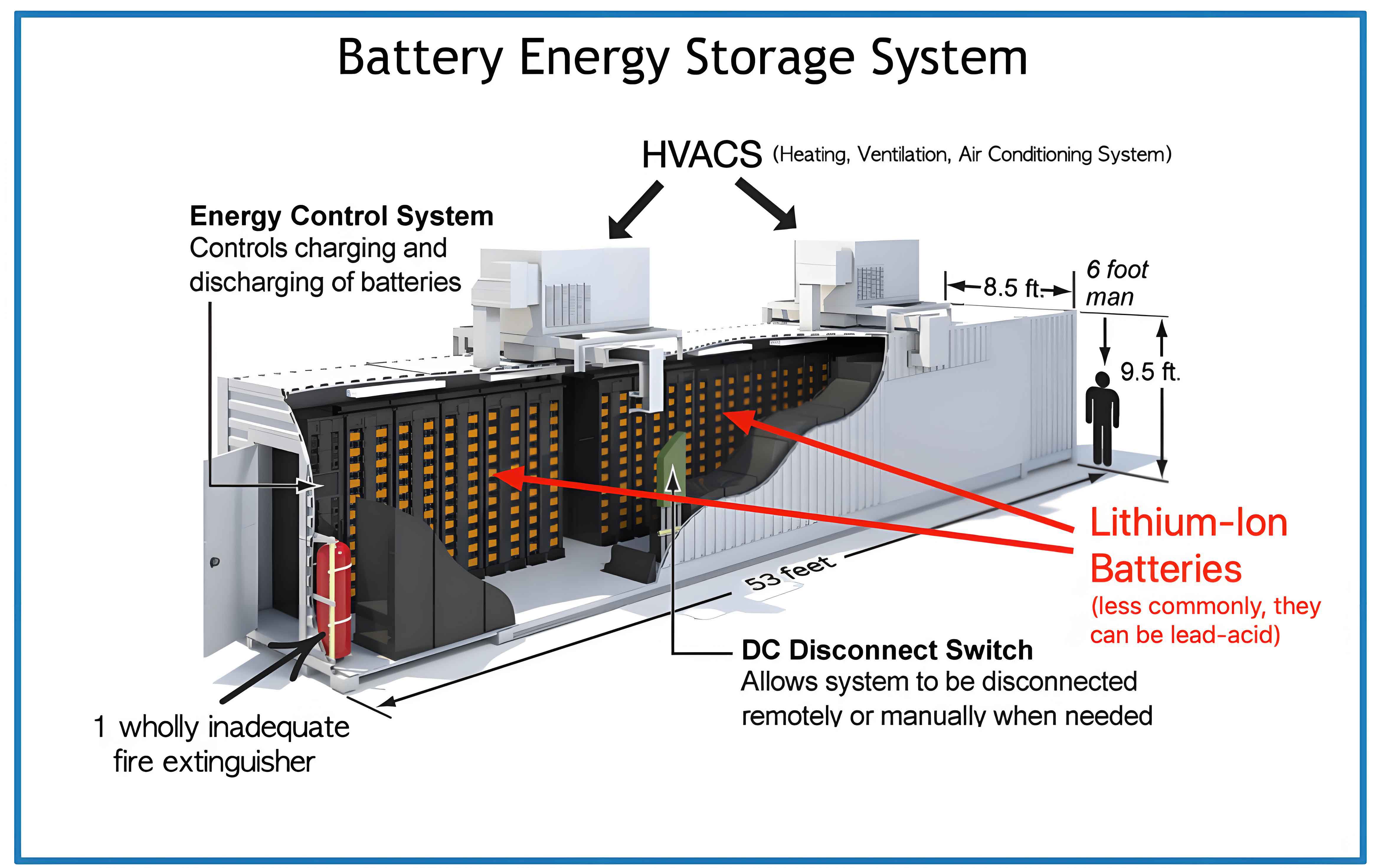
We formulate the optimal configuration of distributed energy storage systems as a multi‑objective bi‑level programming problem. The upper level decides the location and capacity of the energy storage system, while the lower level optimizes the hourly charging/discharging schedule and PV operation. The interaction between the two levels is shown in the diagram (conceptual).
3.1 Upper Level Model
3.1.1 Objective Function
The upper level minimizes the total annual cost considering investment, operation, and energy purchase, over the stochastic scenarios:
$$ \min F_1 = \sum_{k=1}^{K} p_k \left( C_{\mathrm{inf}} + C_{\mathrm{opex}} + C_{\mathrm{con}} \right) $$
where \(p_k\) is the probability of scenario \(k\), and \(K\) is the total number of scenarios. \(C_{\mathrm{inf}}\) is the investment cost of distributed resources (PV and energy storage):
$$ C_{\mathrm{inf}} = \sum_{i=1}^{N_{\mathrm{dev}}} \frac{r(1+r)^n}{(1+r)^n-1} c_{i,k} E_{i,j} $$
where \(c_{i,k}\) is the unit capacity investment cost of device type \(i\) in scenario \(k\), \(E_{i,j}\) is the installed capacity at node \(j\), \(n\) is the economic lifetime, and \(r\) is the discount rate.
\(C_{\mathrm{opex}}\) is the operation and maintenance cost, obtained from the lower level:
$$ C_{\mathrm{opex}} = \sum_{t=1}^{24} \left[ P_{\mathrm{R}}(t) P_{\mathrm{up}}(t) + \sum_{i=1}^{N_{\mathrm{DG}}} C_{i}^{\mathrm{g}}(t) P_{i}^{\mathrm{DG}}(t) + \sum_{i=1}^{N_{\mathrm{store}}} C_{i}^{\mathrm{e}}(t) P_{i}^{\mathrm{store}}(t) \right] $$
where \(P_{\mathrm{R}}(t)\) is the time‑of‑use electricity price from the upper grid, \(P_{\mathrm{up}}(t)\) is the purchased power, \(C_{i}^{\mathrm{g}}(t)\) and \(P_{i}^{\mathrm{DG}}(t)\) are the generation cost and active power output of the \(i\)‑th distributed generator, and \(C_{i}^{\mathrm{e}}(t)\) and \(P_{i}^{\mathrm{store}}(t)\) are the charging/discharging cost and power of the \(i\)‑th energy storage unit.
\(C_{\mathrm{con}}\) is the annual energy cost (purchasing from the grid):
$$ C_{\mathrm{con}} = T_s \sum_{s=1}^{S} \sum_{t=1}^{24} c_{\mathrm{power},t}^{\mathrm{down}} E_{t,s}^{\mathrm{downgrid}} \sigma^{\mathrm{down}} $$
where \(T_s\) is the number of days represented by typical scenario \(s\), \(c_{\mathrm{power},t}\) is the purchase price, and \(E_{t,s}^{\mathrm{downgrid}}\) is the hourly purchased energy.
3.1.2 Constraints
The upper layer must satisfy power balance, generator ramping, and network constraints. The power balance is:
$$ P_{\mathrm{sr}} = \sum_{i=1}^{N_{\mathrm{bus}}} P_{\mathrm{load},i} – \sum_{j=1}^{N_{\mathrm{DG}}} P_{\mathrm{DG},j} – \sum_{k=1}^{N_{\mathrm{store}}} P_{\mathrm{store},k} $$
where \(P_{\mathrm{sr}}\) is the power supplied by the external grid, \(P_{\mathrm{load},i}\) is the load at node \(i\), \(P_{\mathrm{DG},j}\) is the output of the \(j\)‑th distributed generator, and \(P_{\mathrm{store},k}\) is the output of the \(k\)‑th energy storage system (positive when discharging). Other constraints (ramping, line flow limits, reverse power flow) are omitted for brevity.
3.2 Lower Level Model
3.2.1 Objective Function
The lower level aims to minimize a weighted sum of system reliability indices (voltage deviation and load fluctuation) and daily operation cost:
$$ \min F_2 = \sum_{k=1}^{K} p_k \left[ f, \, C_{\mathrm{opex}} \right] $$
where \(f\) combines voltage deviation and load fluctuation:
$$ f = a f_1 + (1-a) f_2 $$
with weighting factor \(a = 0.65\). The voltage deviation is:
$$ f_1 = \sum_{i=1}^{N_{\mathrm{bus}}} \sum_{j=1}^{T_u} |V_{ij} – \bar{V}_i| $$
where \(T_u\) is the number of time intervals in the observation period, \(V_{ij}\) is the voltage at node \(i\) at time \(j\), and \(\bar{V}_i\) is the average voltage at node \(i\).
The load fluctuation is:
$$ f_2 = \sum_{i=1}^{T} \left[ P_{\mathrm{s}}(i) – \bar{P} \right]^2 $$
where \(P_{\mathrm{s}}(i)\) is the input power from the grid at time \(i\), and \(\bar{P}\) is the average input power over the period.
3.2.2 Constraints
- Power limits of devices (e.g., energy storage):
$$ P_{\mathrm{store,min}} \le P_{\mathrm{store}} \le P_{\mathrm{store,max}} $$ - Node voltage limits:
$$ V_{\mathrm{min}} \le V_{ij} \le V_{\mathrm{max}} $$ - Energy balance of storage over the optimization cycle:
$$ \sum_{i=1}^{T} P_{\mathrm{store}}(i) \Delta t = 0 $$ - Other conventional constraints (line capacity, transformer tap limits, etc.) are set according to standard distribution network models.
4. Solution Algorithm – Improved SA‑PSO
We adopt an improved multi‑objective particle swarm optimization algorithm that incorporates the acceptance criterion of simulated annealing. The idea is to allow the algorithm to accept worse solutions with a certain probability during the early stage, thereby enhancing global search ability and avoiding premature convergence. The steps are as follows:
- Obtain the typical scenarios after clustering, including PV power and load at each node and each time.
- Initialize PSO parameters (population size, maximum iterations, etc.) and compute the initial random solution for simulated annealing.
- Randomly select the installation positions and capacities of distributed PV and energy storage systems to form the initial particle swarm. Limit the update velocity and position. Compute the acceptance probability function for SA.
- Evaluate the upper‑level and lower‑level objective functions. Update the personal best and global best of each particle.
- Introduce the SA acceptance criterion: for each new candidate solution, even if it is worse than the current one, accept it with a probability \(\exp(-\Delta E / T_{\text{temp}})\), where \(\Delta E\) is the cost difference and \(T_{\text{temp}}\) is the current temperature. This probability decreases as iterations progress (temperature decreases).
- Transfer the positions and capacities obtained from the upper level to the lower level, and solve the lower‑level operation model using a commercial solver (e.g., Gurobi). Return the operation cost to the upper level.
- Under all constraints, use the total annual cost as the fitness value to update the global best solution.
- Output the optimal configuration scheme.
Compared with the traditional PSO, the SA‑PSO has a higher chance to escape local optima due to the probabilistic acceptance of inferior solutions. The convergence diagram (conceptual) shows that while SA‑PSO may converge later than standard PSO, it achieves a better (lower) objective value and yields a more uniformly distributed Pareto front.
5. Case Study
We test the proposed method on the IEEE33‑node distribution system (base voltage 12.66 kV). Node 1 is the slack node connected to the upper grid, which sells electricity at time‑of‑use prices (see Table 1).
| Period | Time interval | Purchase price (yuan/(kW·h)) |
|---|---|---|
| Peak | 10:00–15:00, 18:00–21:00 | 0.86 |
| Flat | 07:00–10:00, 15:00–18:00, 21:00–23:00 | 0.61 |
| Valley | 00:00–07:00, 23:00–24:00 | 0.30 |
The optimization horizon is 24 hours with a 1‑hour step. We construct the basic scenario set from 8760 hours of historical data. Using the proposed LHS‑based method and the improved K‑means reduction, we obtain 10 typical scenarios. Table 2 lists the normalized PV and load values for each scenario and their probabilities.
| Scenario | PV (pu) | Load (pu) | Probability |
|---|---|---|---|
| 1 | 0 | 0.5647 | 0.013 |
| 2 | 0.8875 | 0.6478 | 0.049 |
| 3 | 0.6456 | 0.6612 | 0.068 |
| 4 | 0.5474 | 0.8967 | 0.213 |
| 5 | 0.6479 | 0.5721 | 0.074 |
| 6 | 0.8121 | 0.4511 | 0.038 |
| 7 | 0.8613 | 0.7054 | 0.027 |
| 8 | 0.8364 | 0.8972 | 0.375 |
| 9 | 0.6813 | 0.9123 | 0.098 |
| 10 | 0.7204 | 0.4577 | 0.045 |
We compare three schemes:
- Scheme 1: With PV and energy storage, deterministic optimization (no multi‑scenario), using SA‑PSO.
- Scheme 2: With PV and energy storage, stochastic optimization with multi‑scenario, using standard MOPSO.
- Scheme 3: With PV and energy storage, stochastic optimization with multi‑scenario, using SA‑PSO.
The candidate PV connection nodes are 7, 16, and 22; the candidate energy storage connection nodes are 18, 19, 26, and 33. Table 3 shows the optimal configuration results.
| Scheme | PV location | PV capacity (kW) | Storage location | Storage capacity (kW·h) | Total annual cost (10⁴ yuan) |
|---|---|---|---|---|---|
| 1 | 7, 11 | 673, 469 | 18, 21 | 906, 843 | 1698.44 |
| 2 | 9, 16, 22 | 972, 359, 541 | 18, 19, 33 | 455, 652, 906 | 1781.78 |
| 3 | 7, 16, 22 | 673, 359, 541 | 18, 19, 33 | 906, 652, 906 | 1719.45 |
From Table 3, we see that Scheme 3 (stochastic with SA‑PSO) achieves the lowest annual cost among the stochastic schemes (1719.45 vs 1781.78), though slightly higher than Scheme 1 (deterministic). This is because considering uncertainty adds constraints that may reduce economic efficiency, but the difference is small, indicating that the proposed model maintains good economy while improving security.
Figure (conceptual) shows the power balance of Scheme 3. The energy storage system charges during valley hours and discharges during peak hours, effectively shaving peaks and filling valleys. The state‑of‑charge (SOC) remains within healthy limits (0.1–0.9).
To evaluate the voltage and load fluctuation performance, we compare Scheme 1 (deterministic) and Scheme 3 (stochastic). The voltage profiles show that both schemes keep voltages within the allowed range (0.95–1.05 pu), but the stochastic optimization yields smoother voltage curves with smaller deviations. The load fluctuation comparison shows that the maximum fluctuation in Scheme 3 is 4.35% (overall < 2.4%), while in Scheme 1 it is 7% (overall < 5%). The stochastic model thus provides better voltage support and load smoothing.
We also compare the clustering performance using the DBI index. For the same target number of reduced scenarios (10), the improved K‑means obtains a DBI of 0.3697, while the conventional K‑means obtains 0.4178 (see Table 4). The lower DBI indicates more distinct and representative clusters, confirming the effectiveness of the improved approach.
| Method | Number of scenarios | DBI |
|---|---|---|
| Improved K‑means | 10 | 0.3697 |
| Conventional K‑means | 10 | 0.4178 |
Finally, we compare the convergence performance of standard PSO and SA‑PSO. The SA‑PSO algorithm requires more iterations to converge (around 170 generations) than standard PSO (around 80 generations), but it achieves a lower final fitness value. Moreover, the Pareto front obtained by SA‑PSO is more uniformly distributed, indicating better diversity and global search capability.
6. Conclusion
This paper has presented a stochastic optimization model for distributed energy storage systems considering uncertainties in PV generation and load demand. The main contributions and findings are summarized as follows:
- The multi‑scenario simulation method based on Latin hypercube sampling and improved K‑means clustering with Kantorovich distance can effectively generate typical scenarios that capture the randomness of source and load. The DBI index confirms the superiority of the improved clustering algorithm.
- The bi‑level multi‑objective model simultaneously considers economy (investment, operation, energy purchase), voltage deviation, and load fluctuation. The lower level optimizes the operation schedule, while the upper level determines the optimal siting and sizing of the energy storage system.
- The proposed SA‑PSO algorithm, which embeds the acceptance criterion of simulated annealing, effectively avoids premature convergence and obtains a more uniformly distributed Pareto front compared to standard MOPSO. The solution precision and stability are improved.
- Case studies on the IEEE33‑node system demonstrate that the stochastic optimization model (Scheme 3) achieves better voltage regulation and load smoothing than the deterministic counterpart, with only a minor increase in annual cost. The total cost of Scheme 3 (1719.45 × 10⁴ yuan) is lower than that of Scheme 2 (1781.78 × 10⁴ yuan), verifying the effectiveness of the hybrid SA‑PSO solver.
- The proper placement and sizing of distributed energy storage systems can significantly enhance the security and efficiency of distribution networks under high PV penetration, providing a practical tool for distribution system planners.
In future work, we will incorporate more detailed models of other distributed energy resources and consider multi‑time‑scale coordinated control strategies to further improve the robustness and economic performance of the energy storage system planning.