
The accurate and reliable estimation of the State of Charge (SOC) for lithium-ion batteries is a cornerstone technology for Battery Management Systems (BMS) in electric vehicles and energy storage systems. SOC indicates the remaining usable capacity, analogous to a fuel gauge, and is critical for preventing overcharge and over-discharge, optimizing energy usage, and ensuring operational safety. Traditional estimation methods often face significant challenges in dynamic operating conditions, where factors like varying load currents, temperature fluctuations, and battery aging introduce nonlinearities and noise. This paper presents a novel fusion algorithm that integrates the Extended Kalman Filter (EKF) with a Long Short-Term Memory (LSTM) neural network to achieve superior estimation accuracy and robustness. The core idea is to leverage the real-time recursive estimation capability of the EKF and augment it with the powerful nonlinear dynamic error compensation provided by the LSTM, creating an end-to-end correction mechanism. The model foundation is a second-order RC equivalent circuit, whose parameters are identified using the University of Maryland battery dataset. Validation under the Federal Urban Driving Schedule (FUDS) and Beijing Dynamic Stress Test (BJDST) profiles demonstrates that the proposed EKF-LSTM fusion algorithm significantly outperforms the standalone EKF, maintaining SOC estimation errors within 1%.
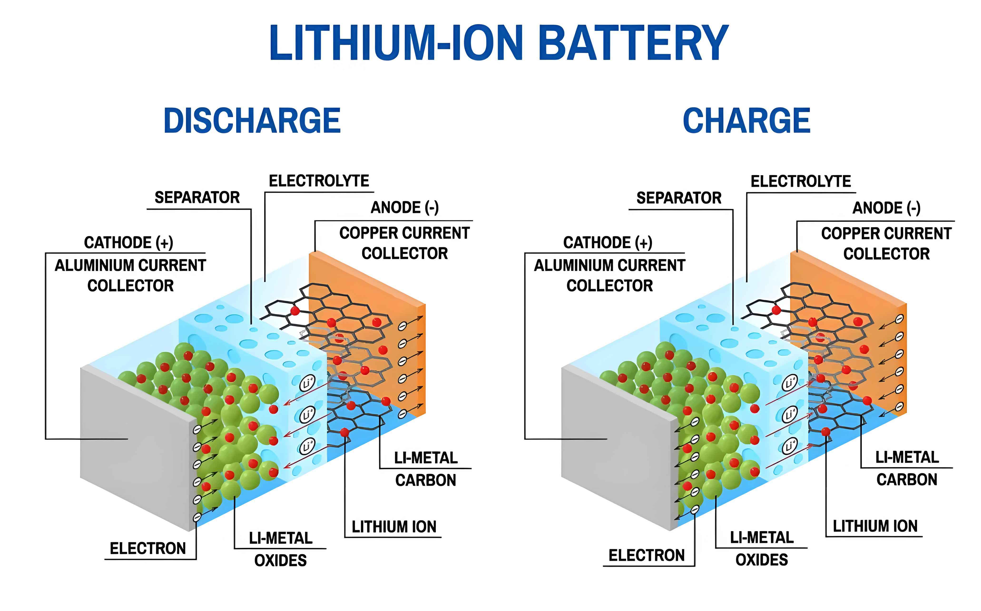
Mathematical Modeling of the Lithium-Ion Battery
An accurate yet computationally efficient model is essential for algorithm development. The second-order Resistor-Capacitor (RC) equivalent circuit model is widely adopted as it effectively captures the dominant dynamic voltage behaviors of a lithium-ion battery, including the instantaneous ohmic drop and the short/long-term polarization effects, without excessive complexity. The model schematic is represented below, where $U_{OC}$ is the Open Circuit Voltage (OCV), $R_0$ is the ohmic internal resistance, $R_1$, $C_1$ and $R_2$, $C_2$ represent the electrochemical and concentration polarization RC pairs, respectively, $I$ is the load current (positive for discharge), and $U_{bat}$ is the terminal voltage.
Applying Kirchhoff’s laws, the continuous-time state-space equations are derived. The state variables are the voltages across the two polarization capacitors ($U_1$, $U_2$) and the SOC itself. The dynamics are described by:
$$
\begin{cases}
\dfrac{dU_1}{dt} = -\dfrac{1}{R_1 C_1}U_1 + \dfrac{1}{C_1}I \\[10pt]
\dfrac{dU_2}{dt} = -\dfrac{1}{R_2 C_2}U_2 + \dfrac{1}{C_2}I \\[10pt]
\dfrac{dSOC}{dt} = -\dfrac{\eta}{Q_n} I
\end{cases}
$$
Here, $\eta$ is the coulombic efficiency (often assumed to be 1 for discharge), and $Q_n$ is the nominal battery capacity in Ampere-hours (Ah). The measurement equation, which relates the internal states to the measurable terminal voltage, is:
$$
U_{bat} = U_{OC}(SOC) – I R_0 – U_1 – U_2
$$
For digital implementation in estimation algorithms, the continuous model must be discretized. Using a sampling period $T_s$, the discrete-time state-space model is formulated as:
$$
\begin{cases}
\mathbf{x}_k = \mathbf{A}_{k-1} \mathbf{x}_{k-1} + \mathbf{B}_{k-1} I_{k-1} + \mathbf{w}_{k-1} \\
y_k = U_{OC}(SOC_k) – I_k R_0 – U_{1,k} – U_{2,k} + v_k
\end{cases}
$$
where $\mathbf{x}_k = [U_{1,k}, U_{2,k}, SOC_k]^T$ is the state vector at time step $k$, $y_k = U_{bat,k}$ is the measurement, and $\mathbf{w}_k$ and $v_k$ are the process and measurement noise, assumed to be zero-mean white Gaussian sequences with covariance matrices $\mathbf{Q}$ and $R$, respectively. The state transition matrix $\mathbf{A}$ and input matrix $\mathbf{B}$ are:
$$
\mathbf{A} =
\begin{bmatrix}
e^{-T_s/(R_1 C_1)} & 0 & 0 \\
0 & e^{-T_s/(R_2 C_2)} & 0 \\
0 & 0 & 1
\end{bmatrix}, \quad
\mathbf{B} =
\begin{bmatrix}
R_1(1 – e^{-T_s/(R_1 C_1)}) \\
R_2(1 – e^{-T_s/(R_2 C_2)}) \\
-\eta T_s / Q_n
\end{bmatrix}
$$
The nonlinearity of the system arises from the $U_{OC}(SOC)$ function in the measurement equation. Accurate modeling of this SOC-OCV relationship is paramount for the performance of any model-based estimator.
Parameter Identification for the Lithium-Ion Battery Model
The fidelity of the equivalent circuit model hinges on precise parameter identification. This process involves determining the OCV curve $U_{OC}(SOC)$ and the values of $R_0$, $R_1$, $C_1$, $R_2$, and $C_2$ at different SOC points. The Hybrid Pulse Power Characterization (HPPC) test data from the University of Maryland dataset for an INR18650-20R lithium-ion battery (2 Ah, 3.6 V nominal) is used for this purpose.
Identifying the SOC-OCV Relationship
The OCV is defined as the terminal voltage after the battery has rested sufficiently for all polarization voltages to decay. The standard method involves discharging the lithium-ion battery by a small percentage of its capacity (e.g., 10% SOC) using a low, constant current, followed by a long rest period (e.g., 1-2 hours). The voltage at the end of the rest period is recorded as the OCV for that specific SOC point. This process is repeated from fully charged (100% SOC) to fully discharged (0% SOC). The collected data pairs $(SOC, U_{OCV})$ are then fitted with a polynomial function. A 7th-order polynomial is often chosen as it provides an excellent balance between fitting accuracy and avoiding overfitting for most lithium-ion battery chemistries.
$$
U_{OCV}(SOC) = \sum_{i=0}^{7} p_i \cdot SOC^i
$$
Where $p_i$ are the polynomial coefficients obtained from the least-squares fitting process. The high coefficient of determination ($R^2 > 0.999$) and low root mean square error (RMSE) confirm the model’s accuracy.
| SOC | OCV (V) |
|---|---|
| 1.00 | 4.176 |
| 0.90 | 4.050 |
| 0.80 | 3.940 |
| 0.70 | 3.840 |
| 0.60 | 3.754 |
| 0.50 | 3.665 |
| 0.40 | 3.626 |
| 0.30 | 3.599 |
| 0.20 | 3.556 |
| 0.10 | 3.478 |
| 0.00 | 3.264 |
Identifying Dynamic Parameters (R0, R1, C1, R2, C2)
The dynamic parameters are extracted from the voltage response during a single current pulse in the HPPC test. The analysis focuses on three distinct regions: the instantaneous voltage drop, the short-term recovery, and the long-term recovery.
1. Ohmic Resistance ($R_0$): This is determined from the instantaneous voltage change at the beginning and end of the current pulse.
$$
R_0 = \frac{(U_{t_0^-} – U_{t_0^+}) + (U_{t_1^+} – U_{t_1^-})}{2|I_{pulse}|}
$$
where $U_{t_0^-}$ and $U_{t_0^+}$ are the voltages immediately before and after the discharge pulse starts, and $U_{t_1^-}$ and $U_{t_1^+}$ are the voltages immediately before and after the pulse ends.
2. Polarization Time Constants and Resistances: After the current pulse ends ($I=0$), the terminal voltage relaxation is governed by the zero-input response of the two RC circuits:
$$
U_{bat}(t) = U_{OC} – I_{pulse} \left[ R_1 e^{-t/\tau_1} + R_2 e^{-t/\tau_2} \right]
$$
where $\tau_1 = R_1C_1$ and $\tau_2 = R_2C_2$. By fitting the relaxation curve $U_{bat}(t)$ with a dual-exponential function of the form:
$$
U_{fit}(t) = a – b e^{-c t} – d e^{-f t}
$$
The model parameters can be identified as:
$$
R_1 = b / |I_{pulse}|, \quad C_1 = 1/(R_1 \cdot c); \quad R_2 = d / |I_{pulse}|, \quad C_2 = 1/(R_2 \cdot f)
$$
This process is repeated at multiple SOC points (e.g., every 10% SOC) to create parameter maps as functions of SOC, which are then used in the online estimator via interpolation.
Core Algorithm Frameworks: EKF and LSTM
The Extended Kalman Filter (EKF)
The EKF is a cornerstone algorithm for state estimation in nonlinear systems. It linearizes the system model around the current state estimate at each time step using a first-order Taylor series expansion. For our discrete-time lithium-ion battery model, the EKF recursion proceeds as follows:
Initialization:
$$
\hat{\mathbf{x}}_{0|0} = E[\mathbf{x}_0], \quad \mathbf{P}_{0|0} = E[(\mathbf{x}_0 – \hat{\mathbf{x}}_{0|0})(\mathbf{x}_0 – \hat{\mathbf{x}}_{0|0})^T]
$$
Prediction Step (Time Update):
$$
\begin{aligned}
\hat{\mathbf{x}}_{k|k-1} &= f(\hat{\mathbf{x}}_{k-1|k-1}, I_{k-1}) = \mathbf{A}_{k-1} \hat{\mathbf{x}}_{k-1|k-1} + \mathbf{B}_{k-1} I_{k-1} \\
\mathbf{P}_{k|k-1} &= \mathbf{A}_{k-1} \mathbf{P}_{k-1|k-1} \mathbf{A}_{k-1}^T + \mathbf{Q}
\end{aligned}
$$
Linearization: The measurement equation is linearized by calculating the Jacobian matrix $\mathbf{C}_k$:
$$
\mathbf{C}_k = \left. \frac{\partial y}{\partial \mathbf{x}} \right|_{\hat{\mathbf{x}}_{k|k-1}} = \left[ -1, \quad -1, \quad \frac{\partial U_{OC}(SOC)}{\partial SOC} \right]_{SOC=\widehat{SOC}_{k|k-1}}
$$
Correction Step (Measurement Update):
$$
\begin{aligned}
\mathbf{K}_k &= \mathbf{P}_{k|k-1} \mathbf{C}_k^T (\mathbf{C}_k \mathbf{P}_{k|k-1} \mathbf{C}_k^T + R)^{-1} \\
\hat{\mathbf{x}}_{k|k} &= \hat{\mathbf{x}}_{k|k-1} + \mathbf{K}_k \left( y_k – \left( U_{OC}(\widehat{SOC}_{k|k-1}) – I_k R_0 – \hat{U}_{1,k|k-1} – \hat{U}_{2,k|k-1} \right) \right) \\
\mathbf{P}_{k|k} &= (\mathbf{I} – \mathbf{K}_k \mathbf{C}_k) \mathbf{P}_{k|k-1}
\end{aligned}
$$
While effective, the EKF’s accuracy is inherently limited by the first-order linearization error and its dependence on the precision of the pre-identified model parameters, which may not hold under all aging and temperature conditions for the lithium-ion battery.
The Long Short-Term Memory (LSTM) Network
LSTM networks are a special class of Recurrent Neural Networks (RNNs) designed to learn long-term dependencies in sequential data. They overcome the vanishing gradient problem of standard RNNs through a gated cell structure. This makes them exceptionally suitable for modeling the complex, history-dependent dynamics of a lithium-ion battery. The key component is the memory cell $c_t$, which is regulated by three gates:
Forget Gate ($f_t$): Decides what information from the previous cell state $c_{t-1}$ to discard.
$$
f_t = \sigma(\mathbf{W}_f \cdot [h_{t-1}, x_t] + \mathbf{b}_f)
$$
Input Gate ($i_t$): Decides what new information from the current input $x_t$ to store in the cell state.
$$
i_t = \sigma(\mathbf{W}_i \cdot [h_{t-1}, x_t] + \mathbf{b}_i)
$$
Cell State Update: Creates a vector of new candidate values $\tilde{c}_t$ and updates the cell state.
$$
\tilde{c}_t = \tanh(\mathbf{W}_c \cdot [h_{t-1}, x_t] + \mathbf{b}_c), \quad c_t = f_t \odot c_{t-1} + i_t \odot \tilde{c}_t
$$
Output Gate ($o_t$): Decides what part of the updated cell state to output as the hidden state $h_t$.
$$
o_t = \sigma(\mathbf{W}_o \cdot [h_{t-1}, x_t] + \mathbf{b}_o), \quad h_t = o_t \odot \tanh(c_t)
$$
Here, $\sigma$ is the sigmoid activation function, $\tanh$ is the hyperbolic tangent function, $\odot$ denotes the Hadamard (element-wise) product, $\mathbf{W}$ and $\mathbf{b}$ are learnable weight matrices and bias vectors, $x_t$ is the input at time $t$ (e.g., current, voltage), and $h_t$ is the hidden state. This structure allows the LSTM to remember relevant long-term context, such as the cumulative effect of past charge/discharge cycles on the present SOC of the lithium-ion battery.
The Proposed EKF-LSTM Fusion Algorithm
The standalone EKF and LSTM each have limitations. The EKF’s performance degrades with model inaccuracy and significant linearization errors in highly nonlinear regimes. The pure data-driven LSTM, while powerful, lacks a physical model foundation, can be sensitive to the quality and scope of training data, and may exhibit poor generalization or transient lag in real-time estimation. Our proposed fusion strategy synergistically combines their strengths to achieve a more robust and accurate SOC estimator for lithium-ion batteries.
The fundamental concept is to use the LSTM as an intelligent, adaptive error corrector for the model-based EKF. The EKF provides a preliminary, physically-grounded state estimate in real-time. However, due to the mentioned limitations, this estimate contains an error $\epsilon_k^{EKF} = SOC_k^{true} – SOC_k^{EKF}$. The LSTM network is trained to learn this complex error pattern directly from operational data.
Algorithm Structure and Workflow:
1. EKF Module: Runs in real-time as described in Section 3.1. At each time step $k$, it consumes the measured current $I_k$ and voltage $U_{bat,k}$ to produce the prior state estimate $\hat{\mathbf{x}}_{k|k-1}$ and the posterior (corrected) estimate $\hat{\mathbf{x}}_{k|k}$, which includes $\widehat{SOC}_k^{EKF}$.
2. Feature Vector Construction: A feature vector $\mathbf{F}_k$ is constructed for the LSTM input. This vector should contain information relevant to the EKF’s instantaneous estimation error. A effective choice is:
$$
\mathbf{F}_k = [I_k, \quad U_{bat,k}, \quad \widehat{SOC}_k^{EKF}, \quad \Delta I_k]
$$
where $\Delta I_k = I_k – I_{k-1}$ captures the recent current change, a key driver of dynamic voltage response and potential EKF linearization error.
3. LSTM Error Compensation Module: A trained LSTM network takes a sequence of the recent feature vectors (e.g., $\mathbf{F}_{k-n}, …, \mathbf{F}_{k}$) as input. Its task is to output the predicted estimation error $\widehat{\epsilon}_k^{LSTM}$ for the current time step.
$$
\widehat{\epsilon}_k^{LSTM} = \text{LSTM}_{\theta}(\mathbf{F}_{k-n:k})
$$
where $\theta$ represents all the trained weights and biases of the LSTM network.
4. Fusion and Final SOC Output: The final, high-fidelity SOC estimate is obtained by adding the LSTM-predicted error compensation to the EKF’s estimate:
$$
\widehat{SOC}_k^{Final} = \widehat{SOC}_k^{EKF} + \widehat{\epsilon}_k^{LSTM}
$$
This architecture establishes a powerful feedback loop. The EKF provides a stable baseline estimate and handles the fundamental state propagation. The LSTM, acting as a meta-corrector, learns to identify and rectify systematic biases and dynamic errors that the EKF alone cannot capture, particularly during sharp load transitions and under conditions where the pre-identified model parameters deviate from their true values. This hybrid approach enhances the overall resilience of the lithium-ion battery SOC estimation system.
Experimental Validation and Results Analysis
To validate the proposed EKF-LSTM fusion algorithm, comprehensive tests were conducted using real-world driving cycle data from the University of Maryland dataset. The tests focused on the INR18650-20R lithium-ion battery at a constant temperature of 25°C. Two dynamic profiles were selected to simulate rigorous operating conditions: the Federal Urban Driving Schedule (FUDS) and the Beijing Dynamic Stress Test (BJDST). For both tests, the initial SOC was set to 80%, and the discharge was performed down to 10% SOC to avoid the highly nonlinear regions at the extremes.
Data Preparation and LSTM Training
The data from each driving cycle was split, with 70% used for training the LSTM network and the remaining 30% reserved for testing the final fusion algorithm. The training dataset for the LSTM was generated by first running the standalone EKF on the training portion of the cycle data. The true SOC (calculated by high-precision coulomb counting on the test bench data) and the EKF’s estimated SOC were used to compute the target error signal: $\epsilon^{train} = SOC^{true} – SOC^{EKF}$. The LSTM was then trained to predict this error sequence based on the corresponding feature vectors $\mathbf{F}$.
The LSTM network was implemented with the following structure: an input sequence layer, two LSTM layers (with 256 and 128 hidden units respectively) to capture temporal dependencies, followed by a fully connected layer and a regression output layer. The Adam optimizer was used with an initial learning rate of 0.001, a mini-batch size of 64, and training was performed for up to 100 epochs with early stopping to prevent overfitting. The mean squared error (MSE) between the predicted and actual EKF error was used as the loss function.
Performance Evaluation and Comparative Analysis
The performance of the standalone EKF and the proposed EKF-LSTM fusion algorithm was evaluated on the unseen test portions of the FUDS and BJDST cycles. The key evaluation metrics were the Root Mean Square Error (RMSE) and the Mean Absolute Error (MAE) of the SOC estimate relative to the reference SOC.
$$
RMSE = \sqrt{ \frac{1}{N} \sum_{k=1}^{N} (SOC_k^{true} – \widehat{SOC}_k)^2 }
$$
$$
MAE = \frac{1}{N} \sum_{k=1}^{N} | SOC_k^{true} – \widehat{SOC}_k |
$$
The results, both in graphical form and summarized in the table below, demonstrate a clear and significant advantage of the fusion algorithm.
Under the FUDS cycle, which features frequent start-stop and acceleration/deceleration events, the EKF-LSTM fusion algorithm successfully tracks the reference SOC with remarkable precision. The terminal voltage estimation is also noticeably improved. The error statistics reveal a substantial reduction in both RMSE and MAE compared to the standalone EKF.
The BJDST cycle, known for its high-rate and highly variable current pulses, presents an even greater challenge. The standalone EKF shows larger deviations, especially during and after severe current transients. In contrast, the EKF-LSTM fusion exhibits superior robustness, effectively compensating for these dynamic errors. The final SOC estimate remains tightly aligned with the true value throughout the test.
| Algorithm | FUDS Cycle | BJDST Cycle | ||
|---|---|---|---|---|
| RMSE (%) | MAE (%) | RMSE (%) | MAE (%) | |
| Standalone EKF | 1.47 | 1.40 | 1.32 | 1.28 |
| Proposed EKF-LSTM | 0.74 | 0.37 | 0.63 | 0.38 |
The table quantitatively confirms the performance enhancement. The fusion algorithm cuts the RMSE by approximately 50% for both driving cycles. More impressively, the MAE is reduced to around 0.4%, which is less than one-third of the EKF’s MAE. This indicates that the LSTM is not only reducing the magnitude of large errors but also consistently improving the day-to-day estimation accuracy. The SOC error is reliably controlled within a 1% bound, meeting the stringent requirement for high-performance BMS applications in electric vehicles powered by lithium-ion batteries.
Conclusion and Future Perspectives
This paper has presented a novel and effective hybrid algorithm for estimating the State of Charge in lithium-ion batteries. By fusing the model-based recursive estimation framework of the Extended Kalman Filter with the data-driven nonlinear dynamic modeling capability of a Long Short-Term Memory network, we have developed a system that overcomes the individual limitations of each approach. The EKF provides a stable, physically-interpretable baseline estimate in real-time, while the LSTM network learns to predict and compensate for the residual errors arising from model inaccuracies and linearization approximations. The synergy between these two components was validated under demanding FUDS and BJDST driving cycles, where the EKF-LSTM fusion algorithm achieved a superior performance, maintaining SOC estimation errors below 1% and significantly outperforming the standalone EKF in terms of both RMSE and MAE.
This work provides a promising new direction for optimizing Battery Management Systems. The proposed framework is general and can be adapted to different lithium-ion battery chemistries and forms. Future research will focus on enhancing the algorithm’s robustness and applicability under more complex real-world conditions. Key directions include: 1) Integrating adaptive mechanisms to handle parameter variations due to battery aging (SOH), 2) Expanding the feature set for the LSTM to include measured or estimated temperature, as the parameters of the lithium-ion battery are strongly temperature-dependent, and 3) Exploring more advanced neural network architectures, such as Attention-based mechanisms or Transformer networks, to potentially capture even more complex temporal dependencies in the lithium-ion battery‘s operational data. The pursuit of such intelligent, adaptive, and highly accurate estimation algorithms remains crucial for unlocking the full potential, safety, and longevity of lithium-ion battery systems in the sustainable energy landscape.