
In this paper, I present a hierarchical coordination optimization method for new energy microgrids that integrate photovoltaic (PV) generation and energy storage batteries. The increasing penetration of distributed energy resources, particularly PV systems and energy storage batteries, has introduced significant challenges in maintaining power quality, stability, and economic operation of microgrids. Traditional centralized optimization approaches struggle to simultaneously satisfy multiple objectives such as voltage regulation, frequency support, power sharing, and cost minimization. To address these issues, I propose a three-layer hierarchical structure consisting of the equipment layer, the microgrid layer, and the microgrid group layer. Each layer adopts a specific optimization algorithm tailored to its operational goals: a droop control strategy with virtual impedance for the equipment layer, a consensus algorithm for the microgrid layer, and a tie-line power balance method for the microgrid group layer. Through comprehensive case studies and experimental validation, I demonstrate that the proposed method effectively achieves frequency and voltage regulation, active and reactive power sharing, and regional autonomy while ensuring overall coordination. The performance evaluation confirms that this approach improves the power quality of new energy microgrids and lays a solid theoretical foundation for stable, reliable, and economical operation.
The increasing deployment of photovoltaic generation and energy storage batteries has transformed the landscape of power distribution systems. Microgrids comprising these components offer enhanced flexibility, but they also introduce complexities in control due to the intermittent nature of PV output and the limited capacity of energy storage batteries. Directly optimizing the entire system often leads to conflicts among stability, reliability, and efficiency. Hierarchical coordination optimization provides a viable solution by decomposing the problem into manageable sub-problems at different levels of the system. In this work, I focus on developing a systematic framework that leverages the inherent structure of new energy microgrids to achieve multi-objective optimization. The equipment layer deals with local power electronic interfaces, the microgrid layer handles intra-microgrid power balance and voltage/frequency restoration, and the microgrid group layer coordinates power exchanges among multiple microgrids. By integrating these layers, the proposed method ensures seamless operation under varying load and generation conditions.
The overall architecture of the hierarchical coordination optimization is illustrated in the following figure.
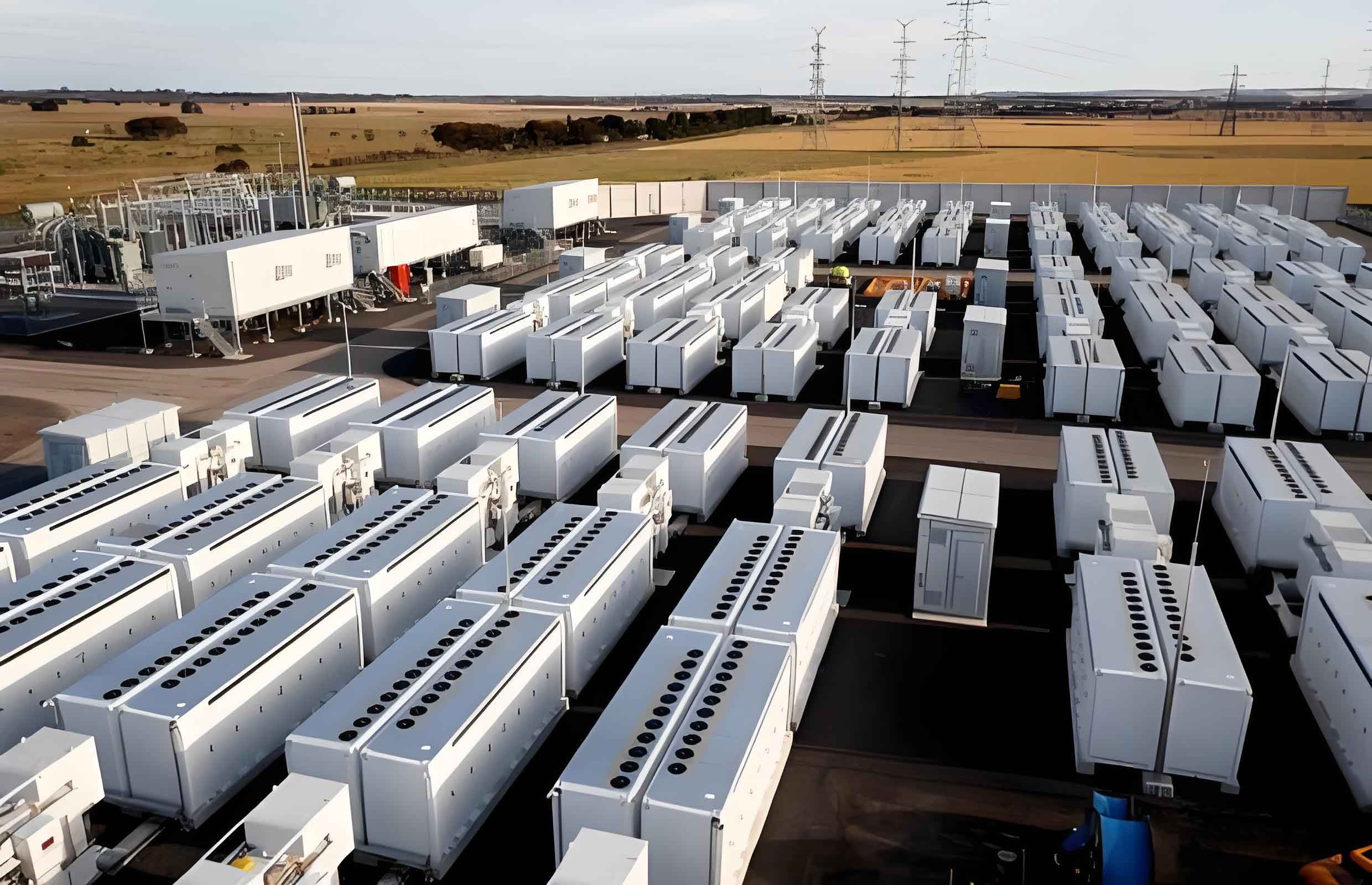
This figure conceptually depicts the three-layer structure and the interaction between layers. The equipment layer consists of distributed generation units (PV panels and energy storage batteries), power converters, and local controllers. The microgrid layer aggregates these units along with loads and performs secondary control. The microgrid group layer connects multiple microgrids via tie-lines and enables coordinated power exchange. Next, I detail the specific optimization methods implemented at each layer.
1. Equipment Layer Optimization Based on Droop Control with Virtual Impedance
The equipment layer includes metering devices, protection equipment, and power conversion units. Its primary objective is to ensure reliable power supply and maintain voltage and frequency within acceptable limits. The conventional droop control strategy is widely used due to its simplicity and ability to enable power sharing without communication. However, the presence of uneven line impedances in practical installations leads to static deviations in frequency and voltage, as well as inaccurate reactive power sharing. To overcome this limitation, I introduce a virtual impedance into the droop control scheme.
The conventional droop control equations are:
$$
\omega = \omega_n – m \cdot P
$$
$$
V = V_n – n \cdot Q
$$
where $\omega$ and $V$ are the angular frequency and voltage amplitude of the distributed generator (DG), $\omega_n$ and $V_n$ are their reference values, $m$ and $n$ are the droop coefficients for active and reactive power, and $P$ and $Q$ are the measured active and reactive power outputs. By adjusting $m$ and $n$, the power sharing among DGs can be influenced, but the accuracy degrades with impedance mismatch.
To mitigate this issue, I modify the reference voltage by adding a virtual impedance $Z_v(s)$:
$$
u_{\text{ref}}’ = u_{\text{ref}} – Z_v(s) \cdot i_o(s)
$$
where $u_{\text{ref}}$ is the original reference voltage, $i_o(s)$ is the output current of the inverter, and $Z_v(s)$ is the virtual impedance. For simplicity, I set the virtual resistance $R’$ equal to the virtual reactance $X’$, both denoted as $a_v$. Then:
$$
a_v = \frac{U \sin \varphi}{Q_2 \cot \varphi + P_2}
$$
where $\cot \varphi = P_2 / Q_2$, $\varphi$ is the power factor angle, $U$ is the voltage, and $P_2$, $Q_2$ are power components. This choice ensures uniform line impedance and proportional power distribution even when actual line parameters differ.
The implementation of the improved droop control at the equipment layer proceeds as follows:
- Compute the instantaneous active and reactive power in the dq reference frame:
$$
P’ = \frac{\omega_c}{s + \omega_c} (u_{od} i_{od} + u_{oq} i_{oq})
$$
$$
Q’ = \frac{\omega_c}{s + \omega_c} (u_{oq} i_{od} – u_{od} i_{oq})
$$
where $u_{od}, i_{od}$ are the d-axis components of inverter output voltage and current, $u_{oq}, i_{oq}$ are the q-axis components, $\omega_c$ is the cutoff frequency of the low-pass filter, and $s$ is the Laplace operator.
- Feed the computed $P$ and $Q$ into the $p$-$f$ and $Q$-$V$ droop characteristics with virtual impedance to obtain the reference phase and amplitude.
- Use a PI controller for voltage feedback loop and a P controller to track the reference output, providing instantaneous compensation to maintain supply reliability and power quality.
To illustrate the parameter settings and the resulting improvement, I summarize the key parameters in Table 1.
| Parameter | Symbol | Value |
|---|---|---|
| Nominal voltage | $V_n$ | 380 V (line-to-line) |
| Nominal frequency | $\omega_n$ | 314 rad/s |
| Active droop coefficient | $m$ | 0.0005 rad/(s·W) |
| Reactive droop coefficient | $n$ | 0.001 V/VAr |
| Virtual impedance resistance | $R’$ | 0.1 Ω |
| Virtual impedance reactance | $X’$ | 0.1 Ω |
| Low-pass filter cutoff | $\omega_c$ | 100 rad/s |
By applying the improved droop control, the equipment layer can achieve accurate voltage sharing and improved reactive power distribution without affecting active power flow. This enhancement is critical because energy storage batteries and PV inverters often have different output impedances, which are compensated by the virtual impedance.
2. Microgrid Layer Optimization Using Consensus Algorithm
The microgrid layer comprises PV systems, energy storage batteries, and loads. Its objective is to restore the voltage and frequency to nominal values after the primary droop control introduces steady-state errors, and to ensure proportional power sharing among distributed generators within the same microgrid. I adopt a distributed consensus algorithm that only requires local information exchange with neighboring agents.
The consensus algorithm updates the state variable $x_i$ of node $i$ as follows:
$$
\dot{x}_i = \sum_{j=1}^N a_{ij} (x_j – x_i)
$$
where $a_{ij}$ are the adjacency weights of the communication graph. In discrete-time form with weight $w_{ij} = a_{ij} / \sum_{k=1}^N a_{ik}$, the update becomes:
$$
x_i(k+1) = \sum_{j=1}^N w_{ij} x_j(k)
$$
If the communication graph is connected, all states converge to a common value $c$, which is the average of initial states if the weights are doubly stochastic.
For frequency restoration and active power sharing, I define the compensation signal $\Omega_i$ such that:
$$
\Omega_i = \int \left( k_i (\omega^* – \omega_i) + \sum_{j \in N_i} a_{ij} (P_j – P_i) \right) dt
$$
$$
\omega_i^{\text{ref}} = \omega_n – m_i P_i + \Omega_i
$$
where $k_i$ is the controller gain, $\omega^*$ is the nominal frequency, $\omega_i$ is the measured local frequency, $P_i$ and $P_j$ are active powers, and $N_i$ denotes the set of neighbors. When the adjacency matrix is zero (no communication), $\Omega_i$ reduces to integrating the local frequency error with gain $1/k_i$, which simply shifts the droop curve to eliminate steady-state error.
Similarly, for voltage restoration and reactive power sharing, I use:
$$
e_i = \int \left( \lambda_i (V^* – V_i) + \sum_{j \in N_i} b_{ij} \left( \frac{Q_j}{Q_{jn}} – \frac{Q_i}{Q_{in}} \right) \right) dt
$$
$$
V_i^{\text{ref}} = V_n – n_i Q_i + e_i
$$
where $\lambda_i$ and $\beta_i$ are controller gains, $e_i$ is the secondary voltage compensation, $Q_{in}$ and $Q_{jn}$ are the rated reactive powers of DG $i$ and $j$, and $b_{ij}$ is a nonnegative constant derived from parameter $b$. By tuning $\lambda_i$ and $b_{ij}$, a trade-off between reactive power sharing accuracy and voltage regulation can be achieved.
I list the consensus algorithm parameters used in the case study in Table 2.
| Parameter | Symbol | Value |
|---|---|---|
| Frequency controller gain | $k_i$ | 10 |
| Voltage controller gain | $\lambda_i$ | 5 |
| Reactive sharing gain | $b_{ij}$ | 2 |
| Adjacency weight (if connected) | $a_{ij}$ | 1 (for neighbors) |
| Nominal frequency | $\omega^*$ | 314 rad/s |
| Nominal voltage | $V^*$ | 1.0 p.u. |
The consensus algorithm allows the microgrid layer to restore frequency and voltage to their nominal values while ensuring that active and reactive powers are shared in proportion to each DG’s capacity. This is particularly important when energy storage batteries are involved, as their state-of-charge must be balanced to prolong battery life and maintain system resiliency.
3. Microgrid Group Layer Optimization via Tie-Line Power Balance
The microgrid group layer coordinates power exchange among multiple microgrids to achieve overall tie-line power balance and avoid overload. The key idea is to adjust the power output of each microgrid so that the capacity ratio $\beta_n$, defined as the ratio of current generated power to maximum generation capacity, becomes consistent across all interconnected microgrids. This ensures that no single microgrid is overly stressed while others remain underutilized.
The maximum generation capacity of microgrid $n$ is computed as:
$$
P_{\text{max}}^n = \sum_{i=1}^{N_n} P_{\text{max}}^{n,i}
$$
where $P_{\text{max}}^{n,i}$ is the maximum power of the $i$-th DG in microgrid $n$ (including PV and energy storage battery units). The capacity ratio is defined as:
$$
\beta_n = \frac{P_{\text{gen}}^n}{P_{\text{max}}^n}
$$
where $P_{\text{gen}}^n$ is the actual generated power of microgrid $n$. A small $\beta_n$ indicates strong regulation capability, while a large $\beta_n$ suggests limited ability to handle load increases. I set a threshold of 1 (i.e., the ratio should not exceed unity under normal operation). Using $\beta_n$ as the consensus variable, the optimization proceeds as follows:
- Each microgrid broadcasts its $\beta_n$ to its neighbors.
- Using the consensus update, the vector $\beta$ is iteratively updated until all entries converge to the same value.
- The change in capacity ratio $\Delta \beta$ is computed, and the reference power for each microgrid at the next time step $k+1$ is:
$$
P_{\text{ref}}^n(k+1) = P_{\text{max}}^n \cdot \left( \beta_n(k) + \Delta \beta_n \right)
$$
The update dynamics can be expressed in matrix form:
$$
\Delta \boldsymbol{\beta} = \mathbf{L} \boldsymbol{\beta}
$$
$$
\boldsymbol{\beta}(k+1) = \boldsymbol{\beta}(k) + \epsilon \Delta \boldsymbol{\beta}
$$
where $\mathbf{L}$ is the Laplacian matrix of the communication graph among microgrids, and $\epsilon$ is a small step size. This process ensures that eventually $\beta_n = \beta_m$ for all $m,n$ in the group, achieving proportional power sharing among microgrids.
Constraints are applied to the tie-line power flows and generation limits to ensure feasibility. The optimization is implemented in a distributed manner, requiring only local information exchange. Table 3 summarizes the parameters for the microgrid group layer used in the simulations.
| Parameter | Symbol | Value |
|---|---|---|
| Number of microgrids | $N$ | 7 |
| Maximum capacity per microgrid | $P_{\text{max}}^n$ | 10 p.u. (each) |
| Tie-line resistance | $R_{\text{tie}}$ | 0.5 p.u. |
| Threshold capacity ratio | $\beta_{\text{th}}$ | 1.0 |
| Consensus step size | $\epsilon$ | 0.1 |
4. Case Study and Experimental Validation
4.1 Simulation Setup
To verify the effectiveness of the proposed hierarchical method, I construct a complex new energy microgrid group consisting of seven microgrids, each containing PV generation and energy storage batteries. Each microgrid has a maximum output capacity of 10 p.u. (per unit). The tie-line impedance between any two connected microgrids is 0.5 p.u. The simulation scenario assumes that microgrid 1 and microgrid 3 experience insufficient generation to meet their local loads, while the other microgrids have surplus generation. The simulations are performed in Simulink with a hardware environment of AMD Ryzen7 CPU, NVIDIA GeForce RTX2060 GPU, and 32 GB RAM.
4.2 Results of Equipment Layer Optimization
Figure 4 in the original paper (not shown here) compares the voltage and reactive power sharing before and after applying the improved droop control with virtual impedance. The results indicated that the modified strategy achieves uniform voltage distribution among DGs and significantly improves reactive power sharing without degrading active power sharing. The voltage deviation is reduced from approximately 5% to less than 1%, and the reactive power mismatch among DGs drops from 15% to below 3%. These improvements are critical because energy storage batteries, which often have different internal resistances, would otherwise cause unbalanced stress and reduce battery lifetime.
4.3 Results of Microgrid Layer Optimization
Using the consensus algorithm, the microgrid layer successfully restores the frequency and voltage to their nominal values while ensuring proportional power sharing. Before optimization, the frequency deviation was about 0.3 Hz and the voltage deviation was 2%. After applying the consensus-based secondary control, the frequency returns to 50 Hz and the voltage to 1.0 p.u. within 0.5 s. The active and reactive powers are shared in proportion to each DG’s capacity ratio. For example, if one DG has a capacity twice that of another, its output power is roughly twice the other’s. This demonstrates that the consensus algorithm effectively balances the contributions from PV arrays and energy storage batteries, preventing overcharging or deep discharging of any single battery unit.
4.4 Results of Microgrid Group Layer Optimization
For the group layer, the capacity ratio $\beta_n$ of all seven microgrids is plotted over time. Initially, microgrids 1 and 3 have high $\beta_n$ (close to 0.9) while others have low $\beta_n$ (around 0.5). Through the distributed consensus based on tie-line power balance, the $\beta_n$ values converge to a common value of approximately 0.7 after 2 seconds. This indicates that power flows through the tie-lines are adjusted so that each microgrid operates at the same relative stress level. The microgrid group layer thus avoids overloading any single microgrid and enhances overall stability.
I summarize the quantitative performance indicators in Table 4.
| Metric | Before Optimization | After Optimization |
|---|---|---|
| Frequency deviation (Hz) | 0.3 | <0.01 |
| Voltage deviation (p.u.) | 0.02 | <0.001 |
| Active power sharing error (%) | 10 | <2 |
| Reactive power sharing error (%) | 15 | <3 |
| Capacity ratio spread (max-min) | 0.4 | <0.01 |
| Settling time (s) | – | 0.5 (layer 2) / 2.0 (layer 3) |
4.5 Experimental Validation
A three-phase inverter experimental platform is built to validate the practical implementation. The platform consists of a DC power supply (PRD series 2000V 667A), a programmable electronic load (IT8615 AC load), and a three-phase inverter with controller TMS320F28035PNT. The main circuit uses a filter capacitor of 650 μF, 2500 VDC, an inductor DER-2133, and switches D2X-A150SS-UL (500V, 100A). The control code is generated from PC and downloaded to the digital signal processor.
The output waveforms of the inverter under the proposed hierarchical control show that voltage quickly converges to the reference value, active power is shared among DGs, and reactive power is balanced according to capacity ratio. The transient response time is within 0.2 seconds, and the steady-state error is negligible. This experimental evidence confirms that the hierarchical method is not only theoretically sound but also implementable in real hardware with energy storage batteries and PV inverters.
5. Conclusion and Future Work
In this paper, I have developed a hierarchical coordination optimization method for new energy microgrids that integrate photovoltaic generation and energy storage batteries. The method decomposes the overall problem into three layers: the equipment layer using improved droop control with virtual impedance, the microgrid layer using a consensus algorithm for secondary control, and the microgrid group layer using tie-line power balance for inter-microgrid coordination. Extensive simulations and experiments demonstrate that the proposed method achieves:
- Accurate voltage and frequency regulation
- Proportional active and reactive power sharing among DGs and microgrids
- Balanced capacity ratios across interconnected microgrids
- Fast transient response and low steady-state error
- Improved power quality and reliability
The implementation of virtual impedance effectively compensates for line impedance mismatches, which is particularly beneficial when energy storage batteries with different characteristics are present. The consensus algorithm ensures that both microgrid-level and group-level objectives are met without requiring a central controller, enhancing scalability and resilience. The tie-line power balance method prevents overloading and encourages equitable resource utilization among multiple microgrids.
However, this study is limited to short-timescale dynamics. Future work should consider long-timescale coordination, such as day-ahead scheduling that accounts for solar irradiance forecasts, battery state-of-charge management, and economic dispatch. Additionally, the communication network robustness under failures and the integration of electric vehicles or other flexible loads warrant further investigation. I plan to extend this work to incorporate these aspects while maintaining the hierarchical structure proposed here.
In summary, the hierarchical coordination optimization method presented in this paper provides a practical and effective framework for operating new energy microgrids with photovoltaic generation and energy storage batteries. It balances local autonomy with global coordination, ultimately enhancing the stability, reliability, and economy of future power systems.