
In modern power electronic systems, the three phase inverter plays a critical role in converting DC power to AC power for various applications, including industrial drives, renewable energy systems, and uninterruptible power supplies. The reliability of these inverters is paramount, as failures can lead to significant performance degradation or even system shutdown. Among the common failure modes, switch open-circuit faults are particularly concerning because they distort output voltages and currents, reduce power quality, and may precipitate secondary faults due to increased stress on remaining components. Traditional fault diagnosis methods often rely on current measurements or complex algorithms, which can be slow, computationally intensive, or require additional hardware. In this article, we propose a novel fault diagnosis method for three phase inverters that leverages the analysis of output voltage trajectories in the αβ plane. Our approach enables rapid detection and precise localization of single or double switch open-circuit faults using only filtered line voltage measurements, making it highly practical and efficient for real-world applications.
The foundation of our method lies in the transformation of three-phase line voltages into the αβ coordinate system using the Clarke transformation. This allows us to visualize the output voltage trajectory, which under normal conditions forms a circular path. When an open-circuit fault occurs in any switch of the three phase inverter, this trajectory distorts in a characteristic manner, providing distinct patterns that correspond to specific fault types and faulty switches. We define several key metrics to quantify these distortions, including the reference radius (Rref), real-time radius (RRT), and deviation degree (DEV), which collectively facilitate fault detection. For fault type identification, we introduce the distance ratio (DR), and for fault localization, we utilize the phase angle (PA) of the average voltage vector or the average sum ratio of line voltages (Avg_Sum(AB/BC)), depending on the fault category. Our method is designed to handle all possible single and double switch open-circuit faults in a three phase inverter, categorizing them into five types for systematic diagnosis.
To elaborate, the three phase inverter topology with an LC filter, as considered in our study, consists of six switches (e.g., IGBTs) with anti-parallel diodes. The output line voltages vAB, vBC, and vCA are measured and processed. We assume a maximum of two simultaneous open-circuit faults, leading to 22 distinct fault scenarios, including the healthy state. These are grouped into five types: Type 0 (no fault), Type 1 (single switch open-circuit), Type 2 (two open-circuit switches on the same side), Type 3 (two open-circuit switches on opposite sides with cross connections), and Type 4 (both switches open in one phase). Each fault type produces a unique voltage trajectory in the αβ plane, which we analyze to derive fault signatures.
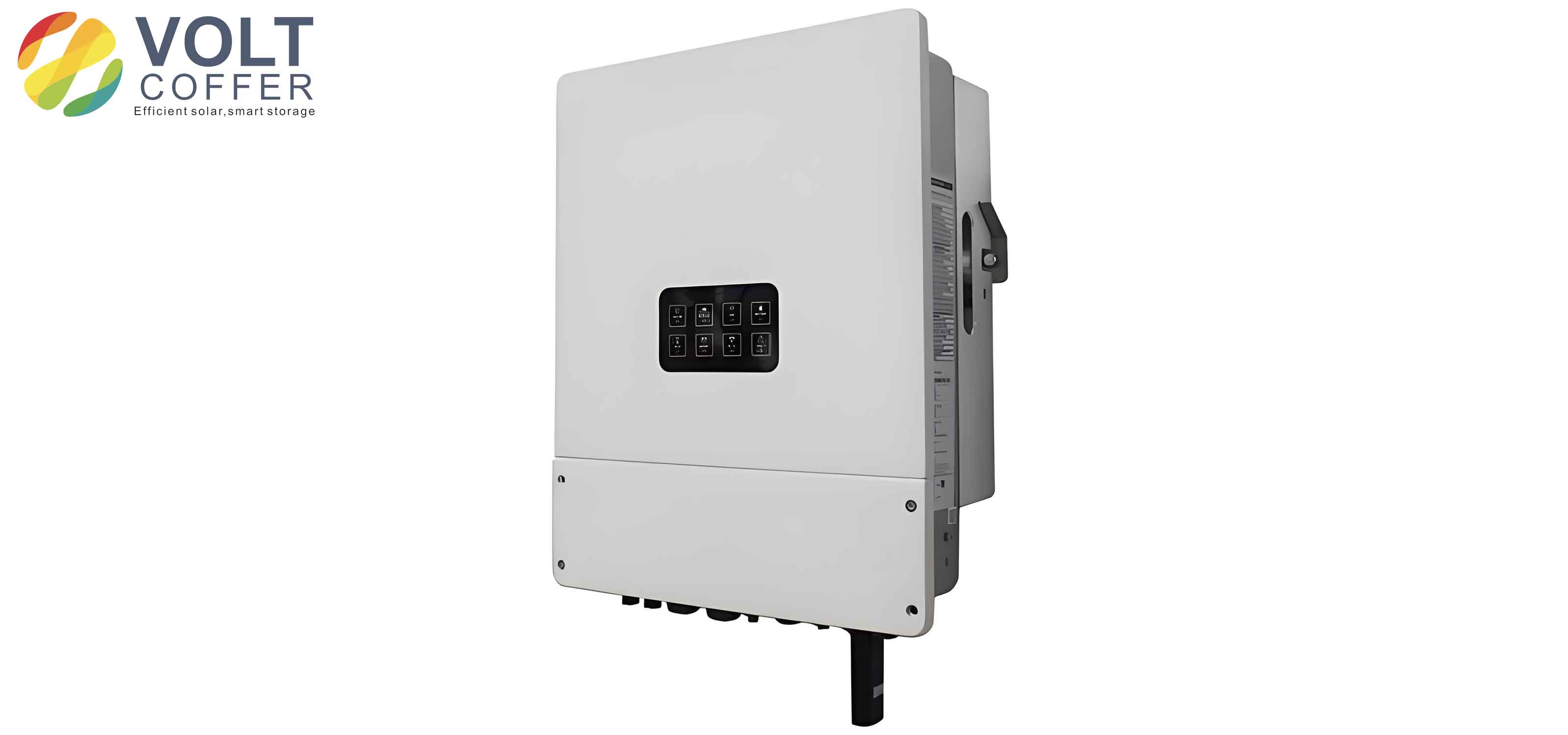
The core of our diagnosis method involves three sequential steps: fault detection, fault type identification, and fault localization. First, we monitor the output voltage trajectory for deviations from the circular reference path. The reference radius Rref is computed from the previous fundamental cycle’s data, representing the radius of the healthy trajectory. For each new set of voltage measurements in the current cycle, we calculate the real-time radius RRT and the deviation degree DEV. If DEV exceeds a predefined threshold, it triggers the fault diagnosis process, indicating a potential open-circuit fault in the three phase inverter. This step ensures that the method responds only to significant trajectory changes, minimizing false alarms.
Mathematically, the Clarke transformation converts the three-phase line voltages to αβ coordinates as follows:
$$ \mathbf{v}_{\alpha\beta}(i) = \begin{bmatrix} v_{\alpha}(i) \\ v_{\beta}(i) \end{bmatrix} = \frac{2}{3} \begin{bmatrix} 1 & -\frac{1}{2} & -\frac{1}{2} \\ 0 & \frac{\sqrt{3}}{2} & -\frac{\sqrt{3}}{2} \end{bmatrix} \begin{bmatrix} v_{AB,m}(i) \\ v_{BC,m}(i) \\ v_{CA,m}(i) \end{bmatrix} $$
where i = 1, 2, …, N, and N is the number of samples per fundamental period. The reference radius Rref is defined as:
$$ R_{\text{ref}} = \frac{1}{N} \sum_{i=1}^{N} \sqrt{(v_{\alpha}^{k-1}(i))^2 + (v_{\beta}^{k-1}(i))^2} $$
where k denotes the current cycle. The real-time radius RRT for the i-th sample is:
$$ R_{\text{RT}} = \sqrt{(v_{\alpha}^{k}(i))^2 + (v_{\beta}^{k}(i))^2} $$
and the deviation degree DEV is given by:
$$ \text{DEV} = \frac{| R_{\text{RT}} – R_{\text{ref}} |}{R_{\text{ref}}} $$
Once a fault is detected, we proceed to fault type identification using the distance ratio DR. This metric is derived from the average voltage vector over one cycle, which shifts in position depending on the fault type. The average voltage vector components are computed as:
$$ \bar{v}_{\alpha} = \frac{1}{N} \sum_{i=1}^{N} v_{\alpha}(i), \quad \bar{v}_{\beta} = \frac{1}{N} \sum_{i=1}^{N} v_{\beta}(i) $$
The distance Dis from the origin to the average vector is:
$$ \text{Dis} = \sqrt{\bar{v}_{\alpha}^2 + \bar{v}_{\beta}^2} $$
and the distance ratio DR is:
$$ D_{R} = \frac{\text{Dis}}{R_{\text{ref}}} $$
We establish thresholds for DR to classify the fault type. For instance, if DR is below a lower threshold, it indicates no fault or a Type 4 fault; if it falls between two thresholds, it suggests a Type 1 fault; and if it exceeds an upper threshold, it corresponds to Type 2 or Type 3 faults. This classification simplifies the subsequent localization step by narrowing down the possible fault scenarios.
For fault localization, we employ different strategies based on the fault category. Category I includes Type 1, Type 2, and Type 3 faults, where the phase angle PA of the average voltage vector is used. The PA is calculated as:
$$ \text{PA} = \begin{cases} \arctan\left(\frac{\bar{v}_{\beta}}{\bar{v}_{\alpha}}\right) & \text{if } \bar{v}_{\alpha} \geq 0, \bar{v}_{\beta} \geq 0 \\ \pi + \arctan\left(\frac{\bar{v}_{\beta}}{\bar{v}_{\alpha}}\right) & \text{if } \bar{v}_{\alpha} < 0 \\ 2\pi + \arctan\left(\frac{\bar{v}_{\beta}}{\bar{v}_{\alpha}}\right) & \text{otherwise} \end{cases} $$
By comparing PA to predefined threshold sets, we can pinpoint the faulty switches. For example, in Type 1 faults, each faulty switch corresponds to a unique PA value, as summarized in the following table:
| Fault Type | Open-Circuit Switch | PA Value (radians) |
|---|---|---|
| Type 1 | S1 | 7π/6 |
| Type 1 | S2 | 3π/2 |
| Type 1 | S3 | 11π/6 |
| Type 1 | S4 | π/6 |
| Type 1 | S5 | π/2 |
| Type 1 | S6 | 5π/6 |
Similarly, for Type 2 and Type 3 faults, we have distinct PA values that allow for precise identification of the faulty switch pairs. Category II, which consists of Type 4 faults, requires a different approach due to the fundamental change in circuit topology. In this case, the three phase inverter effectively becomes a single-phase system, and we use the average sum ratio Avg_Sum(AB/BC) of the line voltages for localization. This ratio is defined as:
$$ \text{Avg\_Sum(AB/BC)} = \frac{1}{N} \sum_{i=1}^{N} \frac{v_{AB,m}(i)}{v_{BC,m}(i)} $$
For Type 4 faults, this ratio takes specific values: -0.5 for S1&S4 open, 1 for S3&S6 open, and -2 for S5&S2 open. By evaluating this ratio against thresholds, we can accurately identify the faulty phase in the three phase inverter.
To validate our method, we conducted extensive simulations and experiments on a three phase inverter system. The simulation parameters included a DC bus voltage of 311 V, filter inductance of 2 mH, filter capacitance of 10 μF, and a switching frequency of 10 kHz. We implemented space vector pulse width modulation (SVPWM) and introduced open-circuit faults by disabling the gate signals of specific switches. The output line voltages were sampled at 20 kHz, and the fault diagnosis algorithm was applied in real-time. The results demonstrated that our method could detect and locate all single and double switch open-circuit faults within one fundamental cycle, with high accuracy and minimal computational overhead.
For instance, in the case of a single switch open-circuit fault (Type 1), the output voltage trajectory distorts into a characteristic pattern with a specific DR value around 0.32. The PA values obtained from experiments closely matched the theoretical predictions, enabling precise fault localization. The following table compares simulation and experimental results for Type 1 faults:
| Open-Circuit Switch | DR (Simulation) | DR (Experiment) | PA (Simulation, radians) | PA (Experiment, radians) |
|---|---|---|---|---|
| S1 | 0.3221 | 0.3195 | 3.6652 | 3.6477 |
| S2 | 0.3224 | 0.3179 | 4.7137 | 4.6972 |
| S3 | 0.3226 | 0.3175 | 5.7608 | 5.7780 |
| S4 | 0.3226 | 0.3189 | 0.5236 | 0.5304 |
| S5 | 0.3226 | 0.3240 | 1.5696 | 1.5530 |
| S6 | 0.3224 | 0.3245 | 2.6168 | 2.6033 |
Similarly, for Type 2 and Type 3 faults, the DR values were consistently around 0.438 in simulations and varied slightly in experiments due to practical imperfections, but remained within the diagnostic thresholds. The PA values allowed for unambiguous fault identification, as shown in the table below for selected cases:
| Fault Type | Open-Circuit Switches | DR (Simulation) | DR (Experiment) | PA (Simulation, radians) | PA (Experiment, radians) |
|---|---|---|---|---|---|
| Type 2 | S1&S3 | 0.4381 | 0.4282 | 4.7157 | 4.7041 |
| Type 2 | S1&S5 | 0.4380 | 0.4354 | 2.6206 | 2.5926 |
| Type 3 | S1&S6 | 0.4383 | 0.4428 | 3.1409 | 3.1246 |
| Type 3 | S3&S4 | 0.4387 | 0.4301 | 0.0003 | 0.0156 |
For Type 4 faults, the Avg_Sum(AB/BC) ratio provided reliable localization, with experimental values closely aligning with simulations. For example, for S1&S4 open, the ratio was -0.5027 in simulation and -0.5060 in experiment; for S3&S6 open, it was 1.0016 in simulation and 0.9936 in experiment; and for S5&S2 open, it was -2.0090 in simulation and -1.9550 in experiment. These results confirm the robustness of our method across all fault scenarios in a three phase inverter.
In conclusion, we have developed a comprehensive fault diagnosis method for switch open-circuit faults in three phase inverters based on output voltage trajectory analysis. Our approach offers several advantages: it requires only line voltage measurements, minimizing sensor costs; it achieves fast diagnosis within one fundamental cycle; and it covers all possible single and double switch faults. The use of the αβ plane transformation and derived metrics like DR and PA provides a clear framework for fault identification and localization. Simulation and experimental validations on a three phase inverter system demonstrate the method’s accuracy and practicality, making it suitable for integration into real-time control systems for enhanced reliability. Future work could explore adaptation to multi-level inverters or integration with fault-tolerant control strategies to further improve the resilience of power electronic systems.
The effectiveness of our method stems from its ability to leverage the inherent characteristics of the three phase inverter under fault conditions. By focusing on voltage trajectories, we avoid the delays associated with current-based methods and the complexity of artificial intelligence algorithms. Moreover, the self-adaptive nature of the reference radius Rref allows the method to accommodate variations in operating conditions, ensuring consistent performance. As three phase inverters continue to be pivotal in modern power electronics, our diagnosis method provides a reliable tool for maintaining system integrity and preventing catastrophic failures. We believe that this approach can be extended to other power converter topologies, contributing to the advancement of fault diagnosis technologies in the field.