
The accurate estimation of the State of Charge (SOC) stands as a paramount objective in Battery Management Systems (BMS), crucial for ensuring the safety, longevity, and reliable performance of lithium-ion batteries. I have found that the fidelity of this estimation is intrinsically linked to the quality of the underlying battery model. Among the various modeling approaches, electrochemical models offer a profound advantage by describing the internal physicochemical states that directly govern the external electrical behavior of a LiFePO4 battery. This intrinsic connection makes them superior for high-accuracy SOC estimation. However, their original formulation, based on coupled nonlinear partial differential equations (PDEs), is computationally prohibitive for real-time BMS applications. Therefore, my focus has been on developing a simplified yet physically meaningful electrochemical model for the LiFePO4 battery, which retains the core dynamics linking internal lithium concentration to terminal voltage, and finally deriving a state-space representation amenable to efficient computer processing and algorithm implementation.
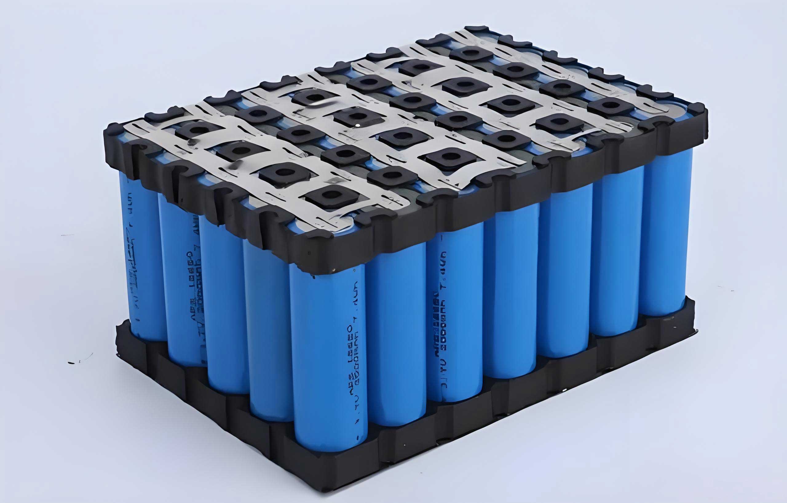
The fundamental physics of a LiFePO4 battery cell can be conceptualized across several domains. Geometrically, we consider a one-dimensional coordinate x spanning from the negative current collector to the positive current collector. Each electrode is porous, filled with active material particles (approximated as spheres) and an electrolyte. Within each spherical particle, a radial coordinate r describes the diffusion of lithium. The primary internal states are the concentration of lithium in the solid phase of the particles, \(c_s(x, r, t)\), and in the liquid electrolyte phase, \(c_e(x, t)\), as well as the potentials in the solid \(\phi_s(x, t)\) and electrolyte \(\phi_e(x, t)\) phases. The external excitation is the applied current \(I(t)\), and the measured response is the terminal voltage \(V(t)\).
The simplified electrochemical model for the LiFePO4 battery is built upon four cornerstone conservation laws, each expressed as a governing equation:
1. Solid-Phase Lithium Diffusion (Fick’s Second Law): This describes how lithium ions move within the spherical active material particles of the LiFePO4 battery electrode.
$$ \frac{\partial c_s}{\partial t} = \frac{D_s}{r^2} \frac{\partial}{\partial r} \left( r^2 \frac{\partial c_s}{\partial r} \right) $$
with boundary conditions:
$$ \left. \frac{\partial c_s}{\partial r} \right|_{r=0} = 0 \quad \text{and} \quad \left. -D_s \frac{\partial c_s}{\partial r} \right|_{r=R_s} = \frac{j}{F} $$
where \(j\) is the pore wall flux of lithium ions (positive during discharge).
2. Liquid-Phase Lithium Conservation (Material Balance): This governs the transport and diffusion of lithium ions in the electrolyte of the LiFePO4 battery.
$$ \epsilon_e \frac{\partial c_e}{\partial t} = \frac{\partial}{\partial x} \left( D_e^{\text{eff}} \frac{\partial c_e}{\partial x} \right) + \frac{a_s j}{F} (1 – t_+^0) $$
with insulating boundary conditions at the current collectors:
$$ \left. \frac{\partial c_e}{\partial x} \right|_{x=0} = \left. \frac{\partial c_e}{\partial x} \right|_{x=L} = 0 $$
3. Solid-Phase Charge Conservation (Ohm’s Law): This describes the electron conduction through the solid matrix of the LiFePO4 battery electrode.
$$ \frac{\partial}{\partial x} \left( \sigma^{\text{eff}} \frac{\partial \phi_s}{\partial x} \right) = a_s F j $$
with boundary conditions linked to the applied current \(I(t)\):
$$ \left. -\sigma^{\text{eff}} \frac{\partial \phi_s}{\partial x} \right|_{x=0} = \left. \sigma^{\text{eff}} \frac{\partial \phi_s}{\partial x} \right|_{x=L} = \frac{I(t)}{A} $$
4. Liquid-Phase Charge Conservation: This governs the ion conduction through the electrolyte of the LiFePO4 battery.
$$ \frac{\partial}{\partial x} \left( \kappa^{\text{eff}} \frac{\partial \phi_e}{\partial x} \right) + \frac{\partial}{\partial x} \left( \kappa_D^{\text{eff}} \frac{\partial \ln c_e}{\partial x} \right) = -a_s F j $$
with boundary conditions:
$$ \left. \frac{\partial \phi_e}{\partial x} \right|_{x=0} = \left. \frac{\partial \phi_e}{\partial x} \right|_{x=L} = 0 $$
These four PDEs are coupled through the Butler-Volmer kinetic equation, which links the reaction current density \(j\) to the surface overpotential \(\eta\):
$$ j = i_0 \left[ \exp\left(\frac{\alpha_a F}{RT} \eta\right) – \exp\left(-\frac{\alpha_c F}{RT} \eta\right) \right] $$
where the overpotential is \(\eta = \phi_s – \phi_e – U(c_{s,\text{surf}})\), and the exchange current density \(i_0\) is:
$$ i_0 = k (c_e)^{\alpha_a} (c_{s,\text{max}} – c_{s,\text{surf}})^{\alpha_a} (c_{s,\text{surf}})^{\alpha_c} $$
Finally, the terminal voltage of the LiFePO4 battery is calculated as:
$$ V(t) = \phi_s(L, t) – \phi_s(0, t) – \frac{R_f}{A} I(t) $$
where \(R_f\) represents contact resistances.
While this “full-order” model provides a high-fidelity description of the LiFePO4 battery, its solution is computationally intensive. The key to practical application in BMS lies in intelligent simplification. The most critical state for SOC in a LiFePO4 battery is the volume-averaged lithium concentration in the solid phase, \(\overline{c_s}(t)\). I approximate the spatial concentration profile within a particle using a parabolic function:
$$ c_s(r, t) \approx a(t) + b(t) \frac{r^2}{R_s^2} $$
By enforcing boundary conditions and the definition of the average concentration, the coefficients \(a(t)\) and \(b(t)\) can be solved. This allows the diffusion PDE to be reduced to an ordinary differential equation (ODE) governing the average concentration. For the negative electrode (which often dictates cell capacity), this simplifies to:
$$ \frac{d \overline{c}_{s,n}}{dt} = – \frac{3 j_{n,\text{avg}}}{R_{s,n} F} $$
A similar equation holds for the positive electrode. The pore wall flux \(j\) is also spatially averaged, simplifying the coupling. Furthermore, the highly nonlinear Butler-Volmer equation can be linearized for small overpotentials, a common approximation in control-oriented models: \( j \approx \frac{i_0 F}{RT} \eta \).
Proceeding with these simplifications for the LiFePO4 battery, and recognizing that for many commercial cells the positive electrode average concentration \(\overline{c}_{s,p}\) is proportional to the negative electrode’s (\(\overline{c}_{s,n}\)), we can combine the thermodynamic open-circuit potentials of both electrodes. The combined open-circuit voltage (OCV) of the LiFePO4 battery, \(U_{\text{ocv}}(\overline{c}_{s,n})\), is a fundamental relationship that can be obtained experimentally and fitted with a high-order polynomial:
$$ U_{\text{ocv}}(x_n) = \sum_{k=0}^{m} p_k x_n^k $$
where \(x_n = \overline{c}_{s,n} / c_{s,n,\text{max}}\) is the normalized stoichiometry in the negative electrode, a direct representation of SOC.
| Model Equation | Full-Order Form | Simplified Form (Control-Oriented) |
|---|---|---|
| Solid Diffusion | PDE: \(\frac{\partial c_s}{\partial t} = \frac{D_s}{r^2} \frac{\partial}{\partial r} \left( r^2 \frac{\partial c_s}{\partial r} \right)\) | ODE: \(\frac{d \overline{c}_s}{dt} = -\frac{3}{R_s F} j_{\text{avg}}\) |
| Butler-Volmer Kinetics | \(j = i_0 [\exp(\frac{\alpha_a F}{RT}\eta) – \exp(-\frac{\alpha_c F}{RT}\eta)]\) | Linearized: \(j \approx \frac{i_0 F}{RT} \eta\) |
| Cell Voltage | \(V = \phi_s(L) – \phi_s(0) – \frac{R_f}{A}I\) | \(V = U_{\text{ocv}}(\overline{c}_{s,n}) + \eta_{\text{polarization}} – \frac{R_{\Omega}}{A}I\) |
Through these steps, the complex distributed-parameter model of the LiFePO4 battery is reduced to a lumped-parameter model centered on the average lithium concentration. This model can be elegantly cast into a discrete-time state-space representation perfect for digital implementation in a BMS:
State Equation (Dynamics):
$$ \mathbf{x}_{k+1} = \mathbf{A} \mathbf{x}_k + \mathbf{B} u_k $$
where the state vector \(\mathbf{x}_k\) typically includes the average lithium concentrations in the negative and positive electrodes (or just the negative one, with the positive deduced by proportionality). The input \(u_k\) is the applied current \(I_k\).
Output Equation (Measurement):
$$ y_k = V_k = U_{\text{ocv}}(x_{n,k}) – R_{\Omega} I_k – R_{\text{ct}} I_k – \text{(Dynamic Polarization Terms)} $$
Here, the output voltage \(y_k\) is a nonlinear function of the state \(x_{n,k}\) (SOC) and the input current \(I_k\). The terms \(R_{\Omega} I_k\) and \(R_{\text{ct}} I_k\) represent ohmic and charge-transfer voltage drops, while additional dynamics from a resistor-capacitor (RC) network are often appended to the state vector \(\mathbf{x}_k\) to capture short-term transient voltage behavior of the LiFePO4 battery.
The following table summarizes the typical parameters required for this simplified LiFePO4 battery model, which can be identified from experimental data.
| Parameter Category | Symbol | Description | Typical Units |
|---|---|---|---|
| Geometric | \(R_s\), \(A\), \(\delta\) | Particle radius, electrode area, thickness | m, m², m |
| Transport | \(D_s\), \(\kappa^{\text{eff}}\), \(D_e^{\text{eff}}\) | Solid diffusivity, electrolyte conductivity, electrolyte diffusivity | m²/s, S/m, m²/s |
| Kinetic | \(k\), \(\alpha_a\), \(\alpha_c\) | Reaction rate constant, anodic/cathodic transfer coefficients | mol/(m²·s·(mol/m³)^(α+1)), – |
| Thermodynamic | \(U_{\text{ocv}}(x)\), \(c_{s,\text{max}}\) | Open-circuit voltage function, max solid concentration | V, mol/m³ |
| Electrical | \(R_{\Omega}\), \(R_{\text{ct}}\), \(C_{\text{dl}}\) | Ohmic resistance, charge-transfer resistance, double-layer capacitance | Ω, Ω, F |
To illustrate the application of this modeling approach for the LiFePO4 battery, consider a standard equivalent circuit model (ECM) enhanced with the electrochemical state. A common and effective structure is the first-order RC model combined with the OCV-SOC relationship derived from the electrochemical model. The combined state-space model becomes:
States: \( \mathbf{x}_k = [z_k \quad v_{c,k}]^T \), where \(z_k\) is the SOC (related to \(\overline{c}_{s,n}\)) and \(v_{c,k}\) is the voltage across the RC polarization branch.
Input: \( u_k = I_k \)
Output: \( y_k = V_k \)
State Update Equations:
$$ z_{k+1} = z_k – \frac{\eta \Delta t}{Q_n} I_k $$
$$ v_{c,k+1} = \exp\left(-\frac{\Delta t}{R_{\text{ct}} C_{\text{dl}}}\right) v_{c,k} + R_{\text{ct}} \left(1 – \exp\left(-\frac{\Delta t}{R_{\text{ct}} C_{\text{dl}}}\right)\right) I_k $$
Output Equation:
$$ V_k = U_{\text{ocv}}(z_k) – R_{\Omega} I_k – v_{c,k} $$
Here, \(Q_n\) is the battery capacity, \(\eta\) is the Coulombic efficiency, and \(\Delta t\) is the sampling time. The function \(U_{\text{ocv}}(z_k)\) is the experimentally-fitted polynomial mapping SOC to open-circuit voltage for the LiFePO4 battery.
In conclusion, the journey from first-principle electrochemistry to a computable state-space model is essential for harnessing the power of physics-based modeling in real-world BMS for LiFePO4 batteries. The simplified electrochemical model I have described successfully captures the critical dynamic relationship between the internal lithium concentration (SOC) and the external terminal voltage, while remaining computationally tractable. This model forms a robust foundation for advanced SOC estimation algorithms like Kalman filters, enabling more accurate, reliable, and safe operation of energy storage systems based on LiFePO4 battery technology. The continuous refinement of these models, coupled with sophisticated parameter identification techniques, remains a vital area of research to push the boundaries of battery management and unlock the full potential of the LiFePO4 battery.
| Model Feature | Full Electrochemical Model | Simplified State-Space Model (for LiFePO4) |
|---|---|---|
| Basis | Fundamental physics (PDEs) | Simplified physics & empirical fits |
| States | Distributed \(c_s(r,x)\), \(c_e(x)\), \(\phi_s(x)\), \(\phi_e(x)\) | Lumped \(\overline{c}_s\) (SOC), polarization voltages |
| Computational Cost | Very High (Finite Element/Volume) | Low (solved in microseconds) |
| Real-Time BMS Suitability | No | Yes |
| Parameter Identification | Complex, requires specialized equipment | Relatively simpler from voltage/current data |
| Primary Use | Cell design, detailed analysis | Online SOC/SOH estimation, control |