
To consider the limitations of grid stability on droop coefficient adjustment, this chapter models the impedance of an inverter system with DC voltage control and solar inverter Q-V droop control in the dq coordinate system. The frequency coupling effect caused by the phase-locked loop and the nonlinearity of the power link are considered, and a complete impedance model of the grid connection port is established; Verify the correctness of theoretical modeling through port frequency sweep; Calculate the determinant zero point of the return matrix to determine the stability of the interconnected system, and further use it as the basis for online stability judgment. Based on this, introduce the secondary adjustment method for the Q-V droop coefficient of the solar inverter and its online application.
1. Impedance modeling and verification
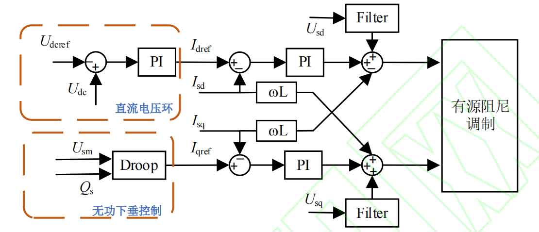
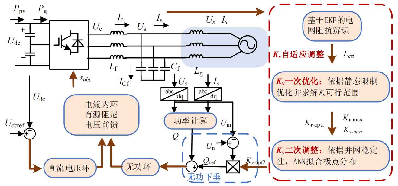
The structure of the grid side inverter control system is shown in Figure 1. The classic phase-locked loop is used to lock the voltage at the grid connection point. The outer loop adopts DC voltage control and voltage reactive droop control, and the inner loop adopts current loop. The main circuit is shown in Figure 2, which, due to the presence of AC capacitors, together with the grid inductance, forms the LCL circuit structure. Here, a relatively simple active damping method is used to suppress the resonant peak. When the DC capacitance is large, the coupling between the front end and the grid side is small and can be ignored. Due to the use of MPPT control in the machine side control structure, the photovoltaic PV side is equivalent to a power source here.
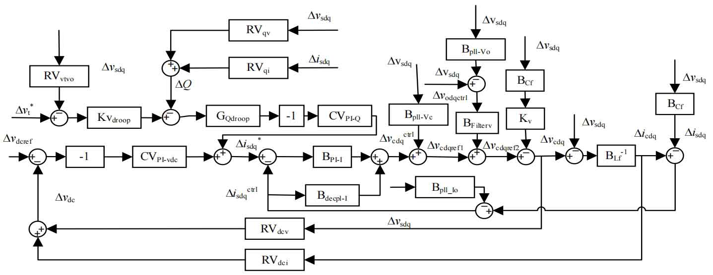
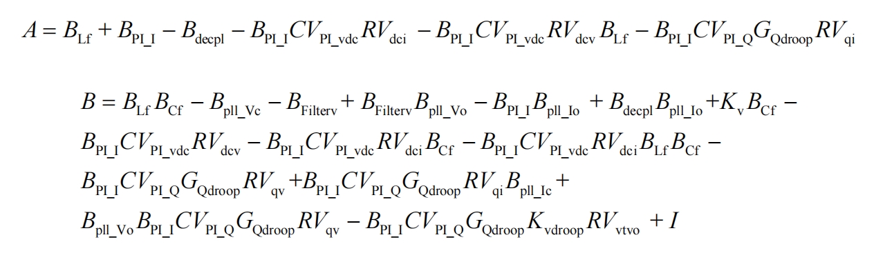
Perform small signal analysis on the system in Figure 1 and draw a small signal modeling diagram of the system as shown in Figure 3. Solve the voltage and current magnitude of the operating point of the system under a given working condition, linearize the system near the operating point, and obtain the control block diagram shown in Figure 3. Solve the relationship between disturbance voltage and disturbance current at the control block diagram port to obtain the expression of the system output impedance. The complete impedance model derivation process considering frequency coupling effect and power nonlinearity is shown in the appendix. The expression for the 2×2 output impedance matrix is shown below. It should be noted that the matrices in the expression are all functions in the s-domain. To simplify the expression, the Laplace operator has been omitted:

Among them:
To verify the correctness of impedance modeling, this paper uses a simulation model to perform frequency sweep verification. Different frequency disturbance voltages are injected under the improved sequence and FFT analysis is performed on the disturbance voltage and current. The frequency sweep results can be calculated using the method proposed in reference. Figure 4 shows the comparison between the frequency sweep results and the theoretical results.
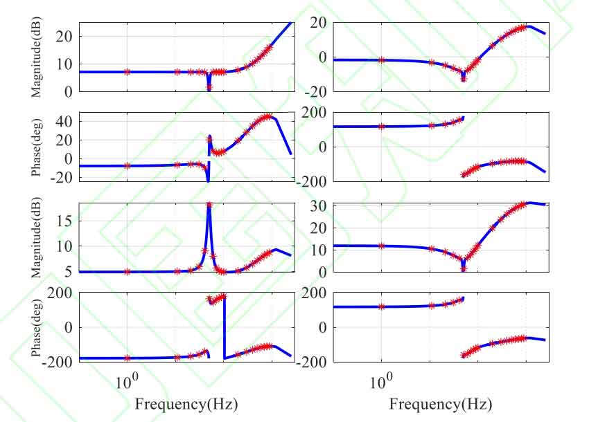
The horizontal axis frequency is the frequency in the abc coordinate system. It can be seen that the impedance matrix is almost consistent with the theory in the frequency range of 1-1000Hz, thus verifying the correctness of the above impedance modeling results.
2. Pole solution and stability assessment of interconnected systems
Based on the previous impedance modeling results, the small disturbance stability of the system can be analyzed and judged. A widely used method for small disturbance stability assessment is the generalized Nyquist criterion. For grid connected converters using grid following control, there is a feedback matrix:
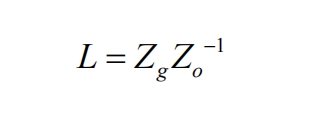
Among them, Zg represents the equivalent impedance of the power grid, and Zo represents the output impedance of the grid connected inverter. Both are 2×2 matrices in the s domain, which is the result of impedance modeling mentioned earlier. Drawing the characteristic root trajectory of the L-matrix and determining whether it surrounds the (-1,0) point can determine the stability of the system.
The proposed adaptive control strategy requires online evaluation of system stability, so the method of solving interconnected system poles is adopted to evaluate system stability. In fact, for converters using grid following control, the generalized Nyquist criterion is equivalent to determining whether the zeros of the following equation are all in the left half plane.
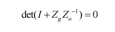
Where I represents the identity matrix of a second-order square matrix. The zero point in the above equation is the pole of the interconnected system. The above equation is a 14th order equation with a total of fourteen zeros. Solving the zeros of the above equation can obtain the poles of the interconnected system.
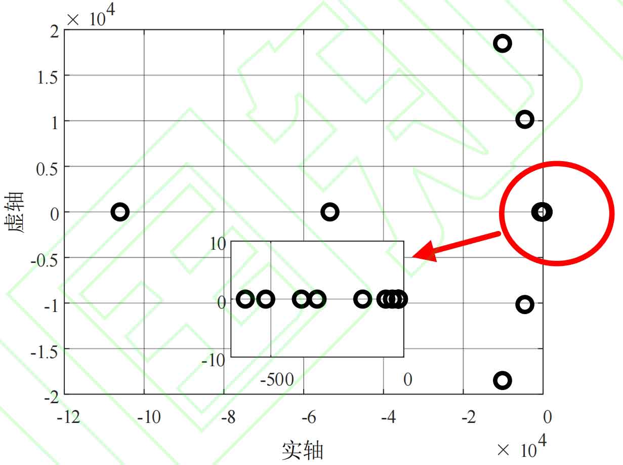
Figure 5 shows the pole distribution of the interconnected system. All poles of the system are distributed in the left half plane, so it can be judged that the system is stable. Since the stability assessment of the system can be summarized as determining whether the pole with the largest real part is distributed in the right half plane, the following section on stability analysis only shows the distribution pattern of the weakest pole of the interconnected system, that is, the pole with the largest real part.
3. Pole mapping learning method for online applications
Due to the fact that adaptive control methods require online assessment of system grid stability, the solution of system poles in stability assessment involves matrix operation, eigenvalue calculation, and higher-order equation solving. To reduce the online computational load of the controller, this article uses an artificial neural network to fit the calculation results of this part of the algorithm. Offline training is conducted using datasets corresponding to system poles with different control parameters, and the trained artificial neural network is used online to predict the small disturbance stability of the system. Due to the fact that this part of the neural network only completes the fitting of existing mapping relationships and requires online real-time operations, the DSP controller has significant limitations on computing power. Therefore, a three-layer fully connected neural network with a relatively simple structure is used for fitting. Drawing a three-dimensional surface based on the weakest pole given by the artificial neural network yields the result shown in Figure 6.
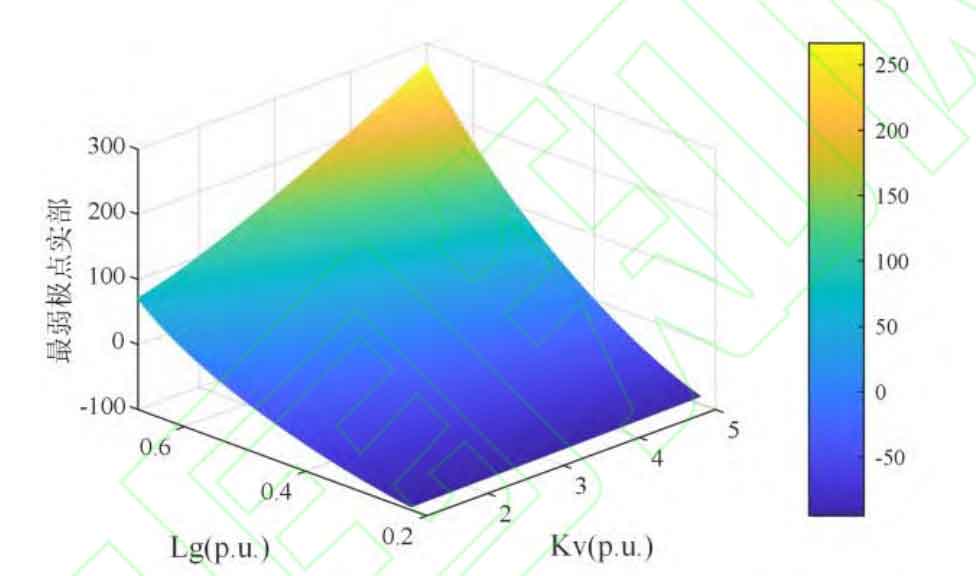
It can be seen that as the inductance of the power grid increases (the strength of the power grid decreases) and the sag coefficient increases, the real part of the weakest pole of the system increases, and the system gradually changes from convergence to divergence. The artificial neural network has obtained the correct variation pattern between the real part of the weakest pole and the sag coefficient, as well as the inductance of the power grid. Within the range of studied parameters, the real part of the weakest pole of the system is positively correlated with the droop coefficient. Therefore, the binary method can be used to optimize the droop coefficient and obtain the set value of the droop coefficient that is closest to the stability margin.
4. Stable control method based on secondary adjustment of Q-V droop coefficient of solar inverter
According to the law of the weakest pole change given earlier, the monotonicity of Kv will not change, so the secondary adjustment of Kv is based on system stability using the binary method. Specifically, as follows:
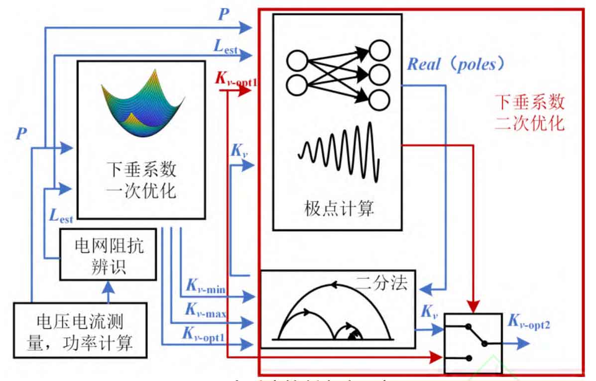
The Q-V droop coefficient secondary adjustment method for solar inverters accepts the first optimization result Kv opt1 as the starting value for stability adjustment and makes stability judgments. If its stability meets the requirements, it can be directly used as a control parameter for control; If its stability does not meet the requirements, solve for the poles at the endpoints of the feasible interval, take the endpoints that meet the stability requirements and the starting value Kv opt1 as the starting interval of the binary method, and use the binary method to solve for Kv opt2 that exactly meets the stability requirements, so that the voltage at the grid connection point is as close as possible to the rated value while meeting the stability requirements. The specific adjustment process is shown in Figure 7.