
From the perspective of system requirements, the anti-interference ability of output voltage is an important indicator to characterize the performance of system design when the load changes. The harmonics of solar inverters usually come from the harmonics generated during PWM modulation, the low order harmonics generated by the dead zone between the upper and lower tubes of the bridge arm, and the low order harmonics generated by the harmonic current of nonlinear loads.
In summary, a qualified solar inverter requires precise control theory to maintain stable output voltage. Among them, the most widely used is the PID control strategy, which has the characteristics of simple structure and mature theory, and is the preferred algorithm for low complexity systems. However, with the increase of human demand, a single PID control strategy cannot meet the high-performance and high-precision control objectives. Therefore, based on the current voltage dual closed-loop control, this system incorporates fuzzy PID control and designs a voltage fuzzy PID control strategy to improve the overall performance of the system.
1. SPWM modulation technology
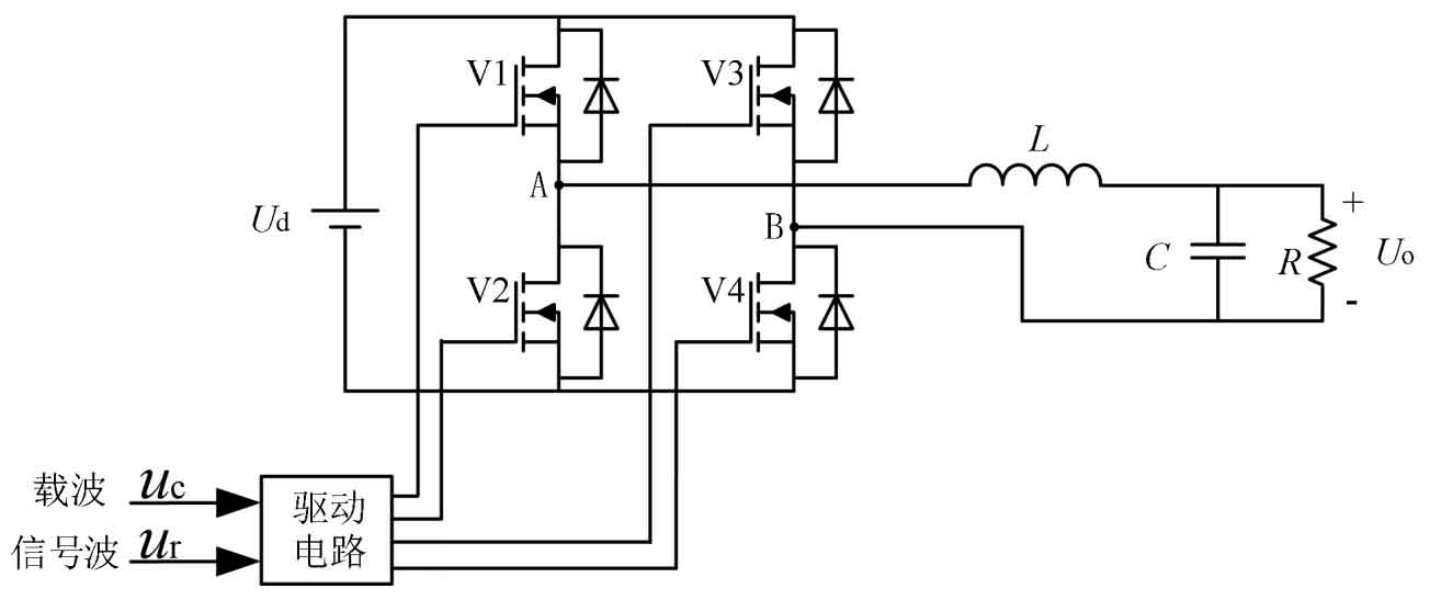
For the inverter part of the DC-AC module, SPWM modulation technology is usually used to control the voltage output of the driving circuit. The control schematic diagram of a single-phase bridge PWM inverter circuit is shown in Figure 1. The pulse signals emitted by the driving circuit control the on/off of four IGBT switching tubes, converting the DC high voltage output from the front stage into AC voltage output.
The basic principle used in SPWM pulse width modulation technology is the principle of area equivalence, which means that when a narrow pulse with equal impulse but different shapes is added to an inertial link, the effect is basically the same. Therefore, the essence of SPWM is to input a pulse sequence with equal amplitude to equivalent a sine wave. Figure 2 shows the waveform of a unipolar PWM control method, and the carrier uc is a positive triangular wave in the positive half cycle of the modulation signal ur, A triangular wave with negative polarity in the negative half cycle of UR.
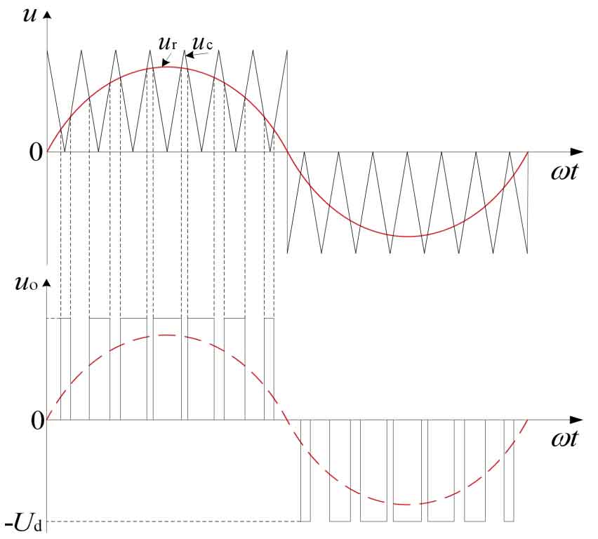
(1) When in the positive half cycle of UR, V1 tube remains in the on state and V2 tube remains in the off state:
When ur>u c, V4 tube conducts and V3 tube turns off, at which uo=Ud.
When ur<u c, the V4 tube is turned off and the V3 tube is conducting, at which point uo=0.
(2) When in the negative half cycle of ur, V1 tube remains disconnected and V2 tube remains on:
When ur<uc, V3 tube conducts and V4 tube turns off, at which uo=- Ud.
When ur>uc, V3 tube is turned off and V4 tube is conducting, at which point uo=0.
Figure 3 shows the waveform of bipolar PWM control mode. In each half cycle of the carrier wave ur, ur has positive and negative, the modulated PWM wave also has positive and negative, and within one cycle of ur, the output is
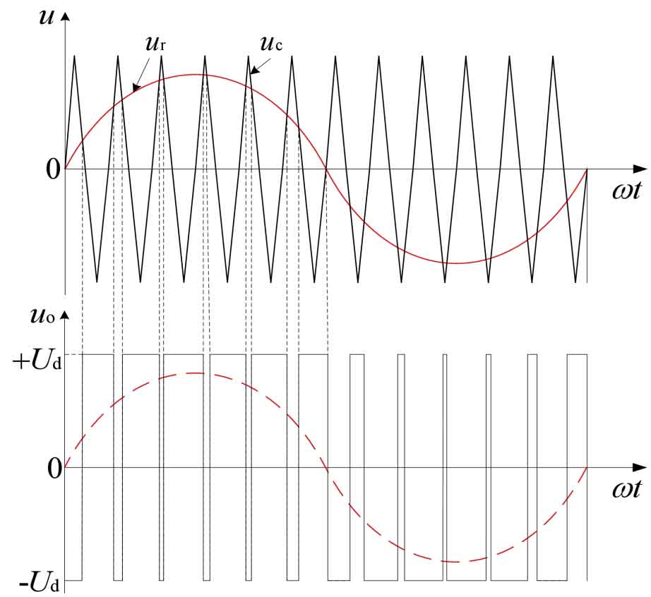
PWM waves only have two levels of ± Ud.
When ur>uc, V1 and V4 pipes conduct, V2 and V3 pipes turn off, and uo=Ud at this time.
When ur<uc, V1 and V4 pipes are turned off, V2 and V3 pipes are conductive, and at this time uo=- Ud.
2. Traditional PID control strategy
2.1 PID control technology
The PID algorithm was the earliest controller used in practical engineering in the field of self-control, and since then, many control algorithms have evolved based on it. The advantage of PID controller lies in its simple structure and principle, without the need to know the precise architecture model of the system in advance.
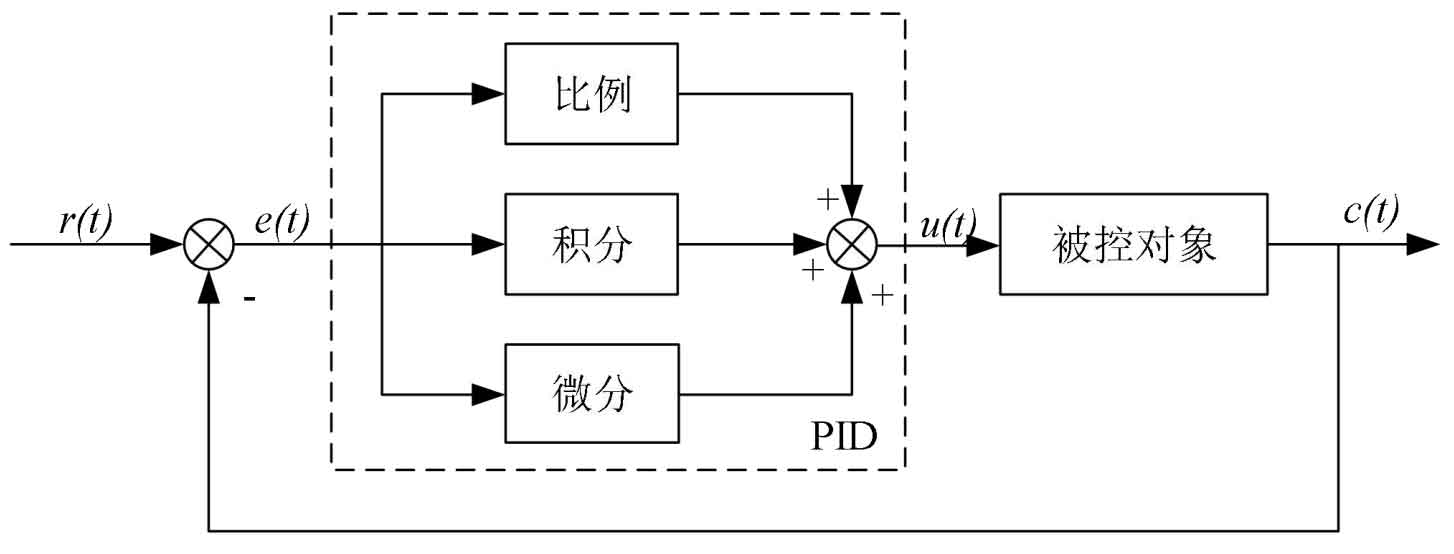
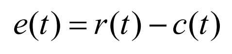
The control principle of a PID controller is to subtract the actual output c (t) from the reference r (t) and obtain a deviation signal e (t), which is sent to the PID controller composed of dashed parts. After corresponding proportional, integral, and differential algorithms are calculated, the output u (t) is then applied to the controlled object, and the actual output c (t) is output by the controlled object, forming a closed-loop structure, Figure 4 is a simple PID control schematic.
The expression for the deviation e (t) is:
Then use the PID controller to calculate the output u (t):
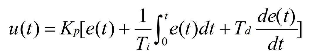
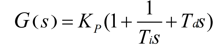
Among them, Kp, Ti, and Td are proportional coefficients, integral time constants, and differential time constants, respectively. After Laplace transformation of the above equation, its transfer function form is obtained:
Below is an introduction to the three key parameters of the PID controller:
(1) Proportional coefficient Kp: Proportional coefficient is a parameter used to improve the response speed of system control. The larger Kp, the more significant the proportional effect, the faster the dynamic response, and the stronger the ability to eliminate errors. However, if the proportional effect is too strong, it can cause system oscillation and deteriorate system stability, and a single proportional adjustment cannot completely eliminate steady-state errors of the system.
(2) Integral time Ti: The principle of integral adjustment is that as long as there is an error, the controller will continue to integrate the error, causing the output to continuously increase or decrease until the steady-state error is zero, and the integration effect stops. However, during the Ti adjustment process, due to the inertia of the actual system, if the integration effect is too strong and the integration output changes too quickly, it may lead to divergent oscillation of the system.
(3) Differential time Td: both proportional and integral adjustment are post adjustment, that is, the system starts to work after the error is generated, while the differential link is used to eliminate the system deviation in advance before the deviation is generated, which greatly improves the dynamic performance of the system.
In summary, if a PID controller wants to control the system to achieve the expected goals, it needs to select appropriate control parameters based on the actual system. Therefore, parameter tuning is particularly important in the design of PID controllers. Generally, tuning methods in engineering include critical proportion method, reaction curve method, and attenuation method.
2.2 Composite control strategy
In complex systems, cascade control is usually adopted to improve the control performance of the system, that is, two controllers are simultaneously used to work in series. Double closed-loop composite control is often used for the control strategy in solar inverters.
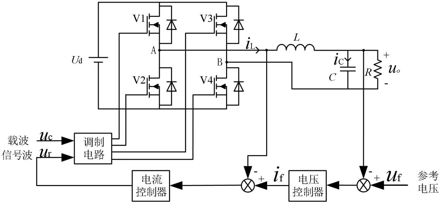
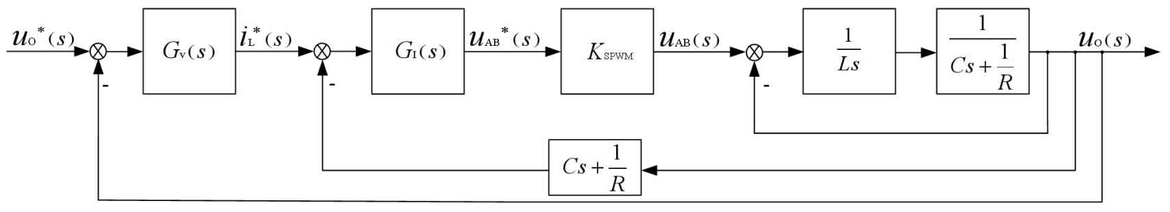
The inverter part of this system adopts voltage and current dual closed-loop control, as shown in Figure 5. The voltage outer loop collects the output voltage and reference voltage, performs a difference operation, and then transmits it to the voltage PID controller. The reference current output by the voltage regulator and the feedback value of the inductance current are subjected to a difference operation, and the operation value is transmitted to the current PID controller. Finally, the current PID controller outputs a signal wave and carrier wave to the modulation circuit, Using SPWM modulation technology to control the on/off of four IGBTs to convert DC voltage into AC voltage output, achieving dual closed-loop composite control of the system.
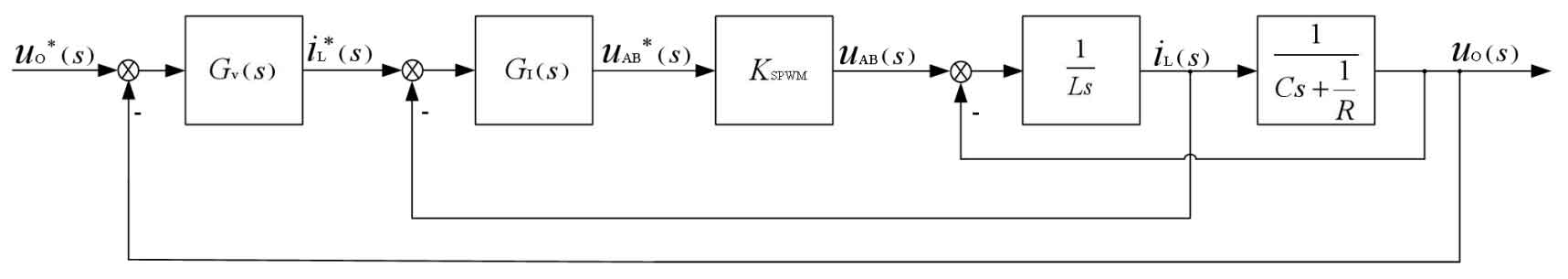
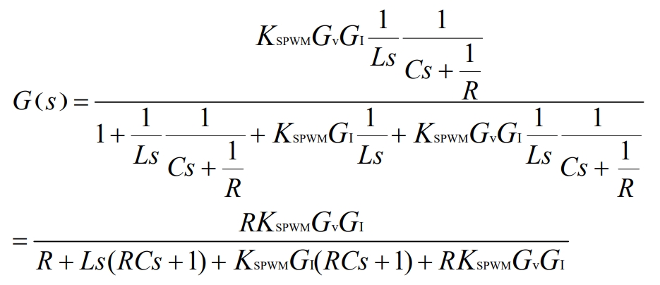
Figure 6 is the control block diagram of Figure 5. After simplifying the flowchart, Figure 7 can be obtained.
According to Mason’s formula, the transfer function is calculated as:
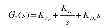
Among them, the transfer function Gv (s) of the voltage outer loop PID controller:
The transfer function GI (s) of the current inner loop PID controller is:
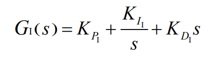
In the formula, the proportional coefficients are KPV and KPI, the integral coefficients are KIV and KII, and the differential coefficients are KDV and KDI.
2.3 Fuzzy Control Theory
The significant advantages of fuzzy control compared to traditional control in practical applications include: no need to obtain accurate mathematical models of the controlled object in advance, enhanced flexibility and maneuverability of system processing, improved contradiction between robustness and sensitivity in control systems, and improved system stability.
2.3.1 Principle and structure of fuzzy controller
The structure diagram of a two-dimensional fuzzy controller is shown in Figure 8. Its principle is to collect the actual value of the controlled quantity from the system signal, and then compare this actual value with the preset value. The compared error signal e and the rate of error change ec are used as inputs to the fuzzy controller. Firstly, the precise values of error e and error rate of change ec are fuzzified to obtain fuzzy quantities. The fuzzy quantities of the two are then subjected to fuzzy inference using the corresponding knowledge base. Finally, the fuzzification is resolved and output to the controlled object.
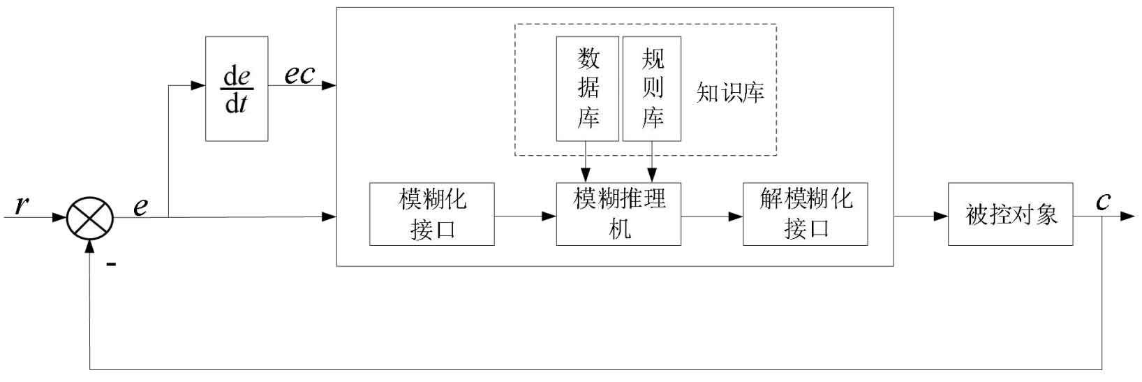
(1) Fuzzy interface
The input received by the fuzzy controller is obtained through fuzzification, so the function of the fuzzification interface is to transform the actual input precise value into an input signal that the fuzzy controller can receive through domain transformation and fuzzification. For a fuzzy input variable, its fuzzy subset can be divided into the following: e={negative large, negative medium, negative small, zero, positive small, positive medium, positive large}={NB, NM, NS, ZO, PS, PM, PB}.
(2) Knowledge base
The combination of database and rule base forms a knowledge base, where the database stores a set of output values corresponding to input values that have been discretized at the domain level. The rule library stores fuzzy control rules, which is a language expression form based on long-term accumulated experience and the operation mode of operators.
(3) Fuzzy inference machine
Fuzzy inference machine is a key step in fuzzy controller, which combines fuzzy rules with fuzzy algorithms, utilizes human thinking, and derives fuzzy control variables from input fuzzy quantities in a reasonable way.
(4) Deblurring
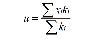
The result obtained after fuzzy reasoning is a fuzzy quantity that cannot be directly used as a control quantity. It must be subjected to deblurring operation, and the main purpose of deblurring is to transform the result of fuzzy reasoning into an analog quantity that can be processed by the executing mechanism. The commonly used methods for resolving fuzziness include maximum membership method, centroid method, and weighted average method:
The maximum membership method is a method of selecting the maximum value by comparing membership degrees. If there is more than one maximum value, it is averaged. Its biggest advantage lies in its simplicity, convenience, and ease of implementation. However, due to only considering the output of the maximum value, it cannot meet the efficiency of control performance in precision control and is not suitable for high-quality systems.
The centroid method is based on the shortcomings of the maximum membership method, and is improved by considering all inputs. The membership degree is enclosed in a graph, and the centroid value is calculated as the output of the entire system. The calculation formula is as follows:
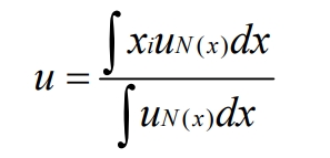
However, in the actual calculation process, due to a large amount of data, it is not possible to calculate all center points. Therefore, further improvements are usually made, such as selecting corresponding representative points for calculation, as shown in the following equation:
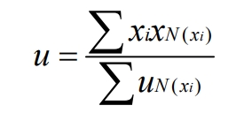
The weighted average rule is commonly used in industrial control, and the output value is determined by the following equation:
2.3.2 Fuzzy controller design method
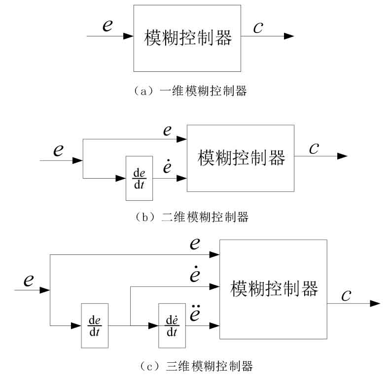
Fuzzy controllers generally have three input variables, namely error, error rate of change, and error rate of change. Figure 9 shows several commonly used structural forms of fuzzy controllers. In theory, the higher the dimension of a fuzzy controller, the more precise the control. Generally, a one-dimensional fuzzy controller can control a first-order controlled object. However, due to the inability of a single control variable to meet the dynamic performance requirements of the system, high-order controllers are commonly used to improve its dynamic performance. However, the establishment of fuzzy rules for high-order controllers is too difficult and difficult to implement. Therefore, two-dimensional fuzzy controllers are currently commonly used for practical control.
(1) Fuzzy set
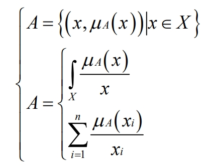
Definition: Let the basic domain be X, where A={X} represents A as its corresponding fuzzy set in X, and its features are represented by μ A: X → [0,1] function representation. The representation of fuzzy sets is as follows:
(2) Membership function
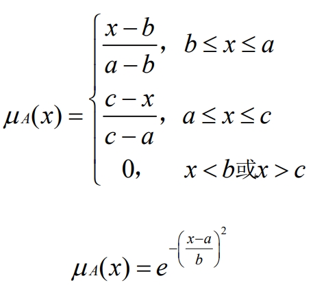
In fuzzy sets, membership functions are commonly used to represent fuzzy concepts. Membership functions can be used to represent a transformation relationship between fuzzy quantities and exact quantities, such as μ A: X → [0,1], when μ The closer the value of A (Xi) is to 1, the greater the degree of belonging to the fuzzy set, and vice versa. At first, due to the convex nature of the membership function, a bell shaped membership function was often used. However, with continuous simplification, trigonometric and normal forms are now commonly used to represent the membership function. The analytical formula for both is shown in the following formula:
(3) Fuzzy relationship
Due to the complexity of fuzzy rules in practical operations, premises and conclusions are often not singular. Both can form their own subsets, and the relationships between the elements in the subset affect each other. In this case, it is necessary to find a comprehensive subset of premises, which is the fuzzy relationship.
Definition: If X and Y are two non empty sets, then a fuzzy subset R of X Å Y is called a fuzzy relationship from X to Y, X Å Y is a Cartesian product, and R is called a fuzzy relationship, determined by the membership function μ A: X Å Y → [0,1] is used to characterize fuzzy relationships.
(4) Fuzzy reasoning
Fuzzy reasoning determines the quality of control effectiveness and is the core of the entire fuzzy controller. The commonly used fuzzy reasoning methods currently include Zadeh method, Larsen method, Mamdani method, etc. Among them, Mamdani method is the most widely used and essentially belongs to synthetic reasoning method.
2.4 Control Algorithm Based on Voltage Fuzzy PID
Due to the fixed and unchanging control parameters of commonly used PID controllers after setting, the harmonic current of the load will generate harmonic voltage drop on the output impedance when the system drives nonlinear loads, causing distortion of the output voltage waveform and affecting the quality of the output voltage. If you want to achieve good control results, it is necessary to constantly adjust the PID parameters for the disturbance at the load end. Adding fuzzy control to PID control can effectively solve such problems.
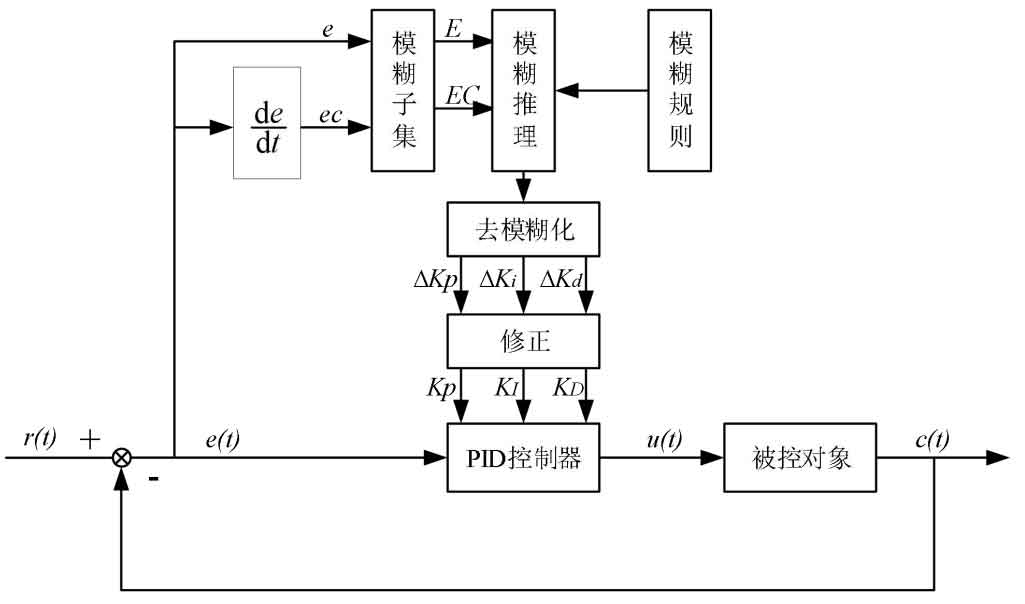
In the traditional voltage current dual closed loop inverter control system, a fuzzy controller is added. By collecting voltage deviation e and voltage deviation change rate ec, the two are used as input signals for the controller. Firstly, the preset fuzzy subset is used to fuzzify the two, and then a series of operations such as fuzzy inference, deblurring, and correction are carried out to improve the Kp of the voltage PID controller KI and KD adjust in real-time based on the current operating status to better control the system output. The overall control principle diagram is shown in Figure 10.
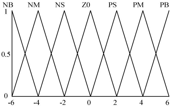
This system uses trigonometric membership functions for fuzzy transformation, and sets the basic universe as a deviation e ∈ X1 ∈ [-6,6], with a deviation change rate ? ∈ X2 ∈ [-1,1]. Multiply the basic domain by the corresponding scaling factors Ke=1 and K ? c=6, so that they are consistent with the fuzzy domain [-6,6]. Select 7 fuzzy subsets, namely “NB”, “NM”, “NS”, “ZO”, “PS”, “PM”, and “PB”. The corresponding relationship of the membership functions is shown in Figure 11.
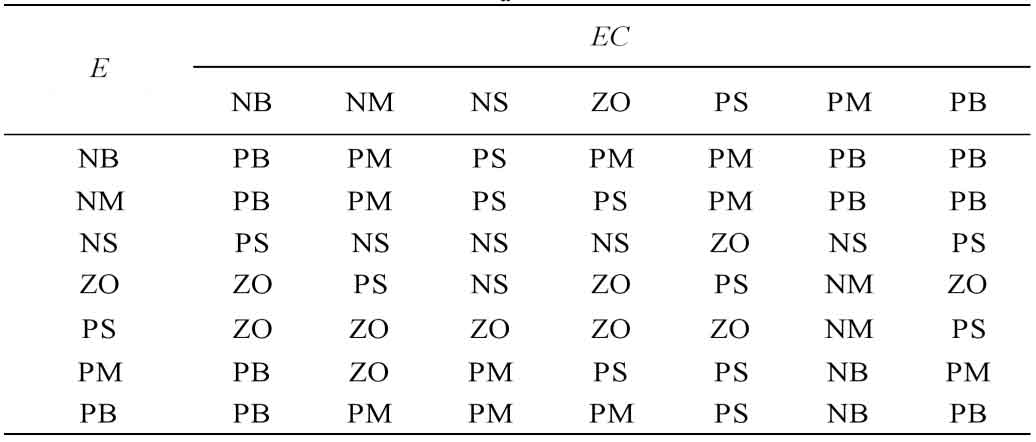
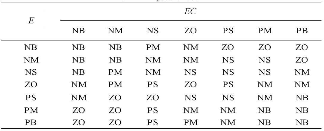
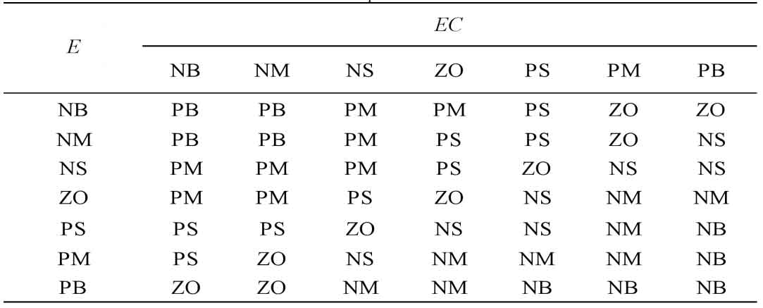
To ensure control effectiveness, fuzzy control tables for ∆ Kp, ∆ Ke, and ∆ kd were developed for the corresponding fuzzy rules and step response of the system, as shown in Tables 1, 2, and 3.
By querying the corresponding fuzzy control rule table, the corresponding fuzzy relationship can be obtained. The maximum membership degree method is used for deblurring operations, and after deblurring, it is corrected. The following equation is the calculation formula:
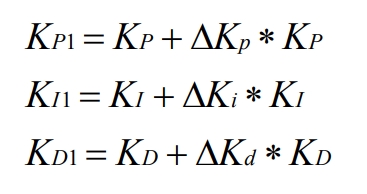
In the formula, KP, KI, and KD are all initial values of the controller parameters, which are obtained through trial and error during pre tuning.
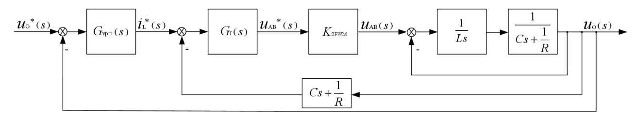
Based on the analysis of the fuzzy control strategy mentioned above, the control algorithm block diagram based on voltage fuzzy PID designed in this article is shown in Figure 12:
Among them, GvpID (s) is a voltage PID controller that has undergone fuzzy control. On the basis of traditional double closed-loop control, fuzzy PID control is introduced to change the parameters of the PID controller, further improving the system’s anti-interference ability, reducing the distortion of the output voltage waveform, and having a good effect on improving the stability of the system.
3. Summary
Based on the key points of system control, the corresponding control strategies are summarized in detail: the FSBB three mode control strategy is used to solve the wide range voltage input demand and the voltage jump problem when the mode changes; The use of voltage fuzzy PID control strategy enhances the control accuracy of the inverter and improves the anti-interference ability when the load changes. This chapter has played a good role in improving the stability of the overall system by studying reasonable control strategies.