
To help achieve the “dual carbon” goal, renewable energy represented by wind power has developed rapidly in recent years. By 2020, the global cumulative installed capacity exceeded 742 GW, and it is expected to reach 56% of the total electricity generation by 2050. Due to the randomness and volatility of wind power, its large-scale grid connection process poses challenges to the safe operation of the power grid. Therefore, configuring energy storage systems in wind farms to alleviate power fluctuations at grid points has become a current research hotspot.
At present, scholars at home and abroad have conducted extensive research on energy storage to suppress wind power fluctuations. On the one hand, algorithms such as low-pass filtering, wavelet packet decomposition, ensemble empirical mode decomposition, and moving average filtering are used to obtain the grid connected components; On the other hand, the battery energy storage system is divided into two parts to independently track fluctuating power and extend its service life by reducing frequent charging and discharging switching. In terms of obtaining grid connected components. Adopting first-order low-pass filtering to smooth the wind power, the high-frequency fluctuations filtered out are compensated by the energy storage system. However, the strong nonlinear characteristics of wind power make it difficult to determine the filtering time constant, and at the same time, there is phase lag during the smoothing process, which increases the energy storage burden by generating trend components. Using wavelet packet decomposition to decompose wind power into three parts: high, medium, and low frequency, and matching power according to the response characteristics of energy storage resources. Propose a wind power smoothing strategy based on adaptive wavelet packets to meet the power smoothing requirements in different fluctuation scenarios. But the effect of wavelet packet decomposition is affected by wavelet basis. The grid connected components are obtained based on ensemble empirical mode decomposition, but the decomposition effect is greatly affected by the decomposition parameters and difficult to select. Obtain grid connected components based on Moving Average Filter (MAF), and determine the length of the filtering window through data prior analysis; Propose an adaptive moving average filter (AMAF) that meets the smoothing requirements to obtain the grid connected components of the grid connected standard. Although the above studies have obtained relatively smooth grid connected components based on different methods, they have not considered the phase lag during the smoothing process, which causes the energy storage system to bear the resulting trend components, increasing its rated power demand and operational burden. Considering the phase lag of the controller, a weighted moving regression filtering strategy based on machine learning is proposed to smooth the photovoltaic power and reduce the phase lag during the control process through a weighting mechanism; We have successively proposed high pass filters (SHF) to reduce phase lag in the wind power smoothing control process, and designed filtering parameters based on power system model parameters. Although the above methods consider the phase lag of the control process, the parameter design is based on data prior analysis, and does not have adaptive adjustment ability during the smoothing process. When the wind power is relatively stable, the energy storage system also needs to be frequently put into operation, increasing its burden.
The battery energy storage system is divided into two independent control groups. The dual lithium battery supercapacitor energy storage system is used to suppress wind power fluctuations, and the lithium battery is divided into two parts to independently undertake charging and discharging tasks to reduce life loss. However, in actual operation, the supercapacitor has already suppressed high-frequency components, and the lithium battery is only used to suppress low-frequency components that change slowly, not fully leveraging the advantages of dual lithium batteries. Reference [18] uses a dual battery energy storage system to alleviate wind power fluctuations, with one set of energy storage used to store power and the other set of energy storage used to transmit power to the grid. When a certain set of energy storage SOC reaches the boundary, the two sets of energy storage charging and discharging modes are converted to reduce the impact of frequent charging and discharging switching on lifespan. However, wind power is transmitted to the grid by the energy storage system, which puts higher requirements on its capacity. A dual battery energy storage system model was built based on PSCAD/EMTDC, and a control strategy for operating at a given discharge depth was proposed. Propose a dual battery energy storage system control strategy based on MPC, and verify that this mode can effectively extend battery life by comparing actual wind power data with a single battery. However, the above research did not consider the imbalance of charge and discharge energy during the suppression process, which may cause the battery energy storage system to operate in high/low SOC extreme situations. In addition, although the operating state of battery energy storage is improved by changing the filtering time constant, the strong nonlinear characteristics of wind power make it difficult to determine the filtering constant to balance the contradiction between power smoothing requirements and SOC optimization in each stage. At the same time, there is phase lag in the control process, which greatly increases the imbalance of charging and discharging energy, posing challenges to battery energy storage SOC control.
A battery integrated energy storage control strategy based on double-layer coordinated control is proposed to address the shortcomings of the above research. In the outer control, the phase lag characteristics of the filter were analyzed in the frequency domain, and a near zero phase filter combining power prediction information was constructed. Subsequently, based on meeting the current grid connection standard, the optimal window length was adaptively determined. For the grid connected components that still do not meet the requirements after using the maximum window smoothing, constraint intervals were used for correction, and a near zero phase adaptive filter for smooth wind power was constructed, This reduces the additional components generated by phase lag and oversmooth in the energy storage power, thereby reducing the rated power demand and operational burden of the energy storage system. In the inner layer control, dual lithium iron phosphate batteries with different charging and discharging characteristics are integrated to track power instructions, and equivalent SOC indicators are defined to measure the overall SOC state of the energy storage system. Subsequently, the equivalent SOC is linked to the outer layer control, and a Logistic dynamic interval based SOC optimization strategy is proposed to meet the requirements of grid connected power during the optimization process, and to solve the extreme operating states of high/low SOC. At the same time, the two batteries can approach the optimal DOD operation, Improve cycle life utilization while ensuring the ability of subsequent batteries to suppress power fluctuations. Finally, the effectiveness and superiority of this strategy were verified based on actual wind power data.
1. Integrated Energy Storage System (IESS) for Suppressing Wind Power Fluctuations
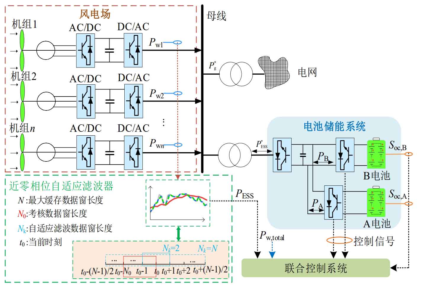
Figure 1 shows the architecture of the wind storage system, Pw1, Pwn is the output of n grid connected fans, PESS and P * ESS are the IESS power reference values and the actual values after considering operational constraints, and P * g is the actual grid connected power. For IESS, this article adopts a long-lived lithium iron phosphate battery, which is divided into two parts with equal capacity for integration, denoted as A battery and B battery. PA and PB represent the energy storage output of the two batteries.
As analyzed in Appendix A, the operating SOC range of IESS is taken as 0.1-0.9. During operation, A/B batteries independently perform charging and discharging tasks to reduce the impact of frequent charging and discharging on battery life, and provide SOC feedback to the control system. Taking A battery charging to suppress positive fluctuations and B battery discharging level to suppress negative fluctuations as an example, switching between charging and discharging at once is as follows: A battery charging to Soc, A=0.9 or B battery discharging to Soc, B=0.1, switching between the two battery charging and discharging modes. When a certain battery cannot completely suppress the fluctuation due to rated power or SOC constraints, it is compensated by another battery. For the extreme operation of IESS with high/low SOC caused by imbalanced total energy of charge and discharge, corresponding SOC reconstruction strategies will be proposed in the future.
1.1 Mathematical model for grid connection of wind storage system
As shown in Figure 1, with the power flow direction to the grid connected busbar as the positive direction, the mathematical model of the wind storage system grid connection is shown in the formula.
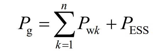
In the formula, Pg is the reference grid connected power; Pwk is the output of the kth typhoon; PESS is the IESS reference power.
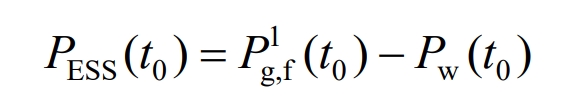
Considering the rated power and SOC constraints during the operation of IESS, the actual grid connected power is shown in the formula. Furthermore, the relationship between the grid connected power reference value and actual value, as well as the IESS power reference value and actual value, can be obtained as shown in the formula.
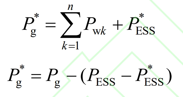
In the formula, P * ESS is the IESS power considering operational constraints; P * g is the actual grid connected power.
During this process, IESS needs to meet: 1) the rated power meets the maximum flat power demand; 2) The rated capacity meets the maximum cumulative suppressed energy demand; 3) SOC is maintained in good condition to ensure that battery energy storage completely suppresses power fluctuations, thereby ensuring that the actual grid connected power meets the requirements. Usually, the maximum suppression power is greater than the maximum cumulative suppression energy, and when configuring the capacity of the battery energy storage system, it is generally based on the C-rate principle. Therefore, meeting 1) and 3) can effectively suppress wind power fluctuations.
1.2 Grid connection standard mathematical model
In order to reduce the impact of random fluctuations in wind power on the power grid, the current national standard proposes limits for active power changes in the 1 minute and 10 minute time scales for grid connected wind power, which are later referred to as wind power smoothing requirements (WPSRs) and are reflected in terms of volatility, as shown in the formula.
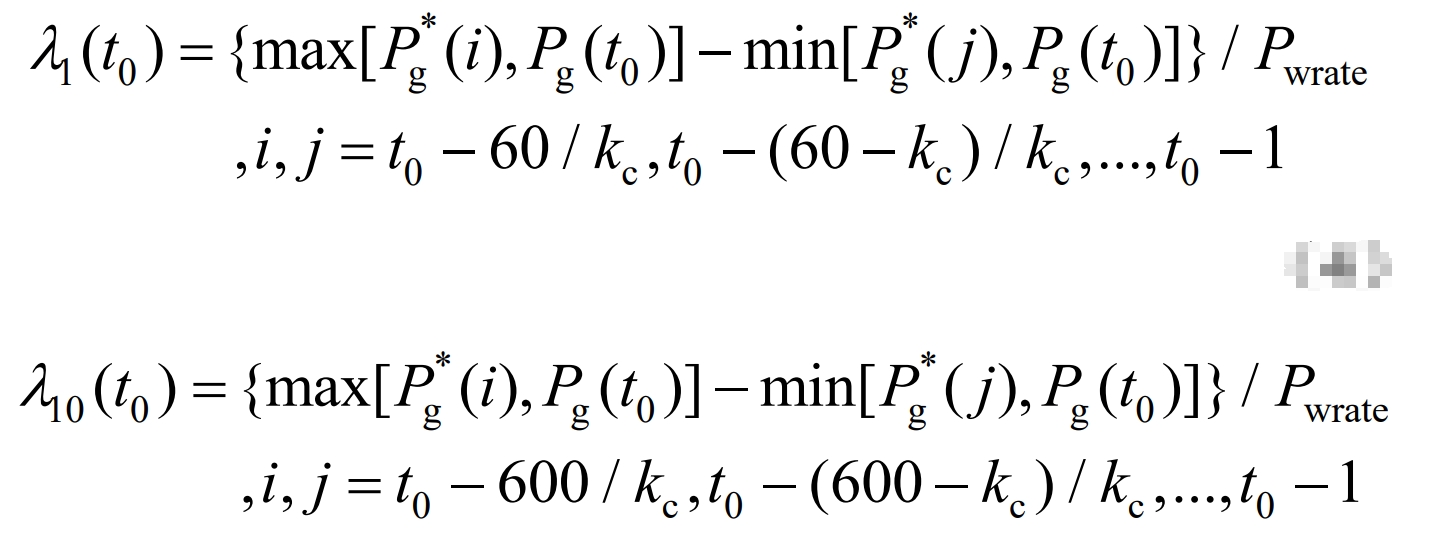
In the equation, λ 1 (t0) λ 10 (t0) is the 1 minute and 10 minute volatility at time t0; Pwrite is the installed capacity of wind power; Kc is the sampling interval. Calculate the volatility at time t0 using a formula and satisfy the λ 1 (t0) ∈ [0,1/10] λ Based on 10 (t0) ∈ [0,1/3], the length of the filtering window is controlled to smooth the wind power and obtain grid connected power that meets WPSRs. The fluctuating power is absorbed by IESS.
Double layer coordinated control of battery energy storage system for suppressing wind power fluctuations
2. Wind power smoothing based on near zero phase adaptive filtering
2.1 Wind power smoothing based on moving average filtering
MAF is a mathematical representation of low-pass filtering, widely used in power smoothing. It caches historical wind power data based on the concept of data windows, calculates the average value of the cached data as the current grid connected power, and then moves the data window to update the data at sampling intervals to achieve wind power smoothing. The mathematical model is:
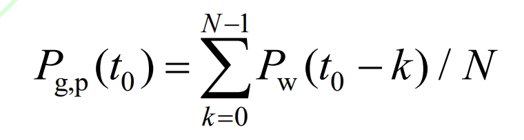
In the formula, Pg and p are the grid connected power after MAF smoothing; Pw is the total output of the wind turbine; N is the length of the data window.
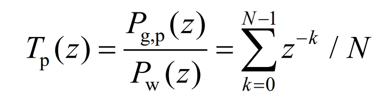
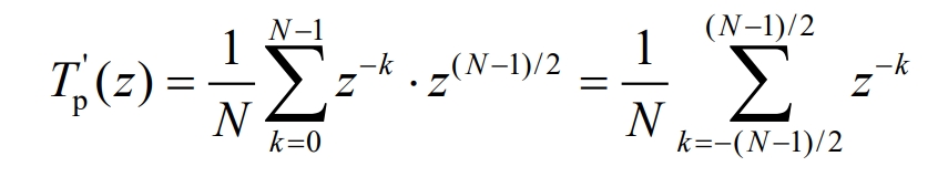
When the data window is larger, the smoothness of the grid connected power is higher, which means that the IESS bears more fluctuating power and greater burden. Therefore, it is sufficient to determine the appropriate data window so that the grid connected power meets WPSRs. Analyze the phase characteristics of the smoothed grid connected power and perform a z-transform on the formula to obtain the transfer function, as shown in the formula.
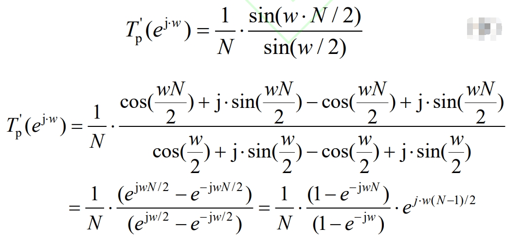
Furthermore, by substituting z=e ^ j · w into the formula, the frequency domain expression can be obtained as:
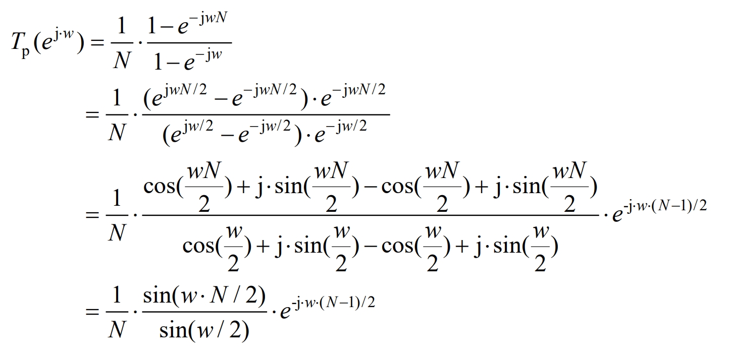
In the formula, w is the angular frequency.
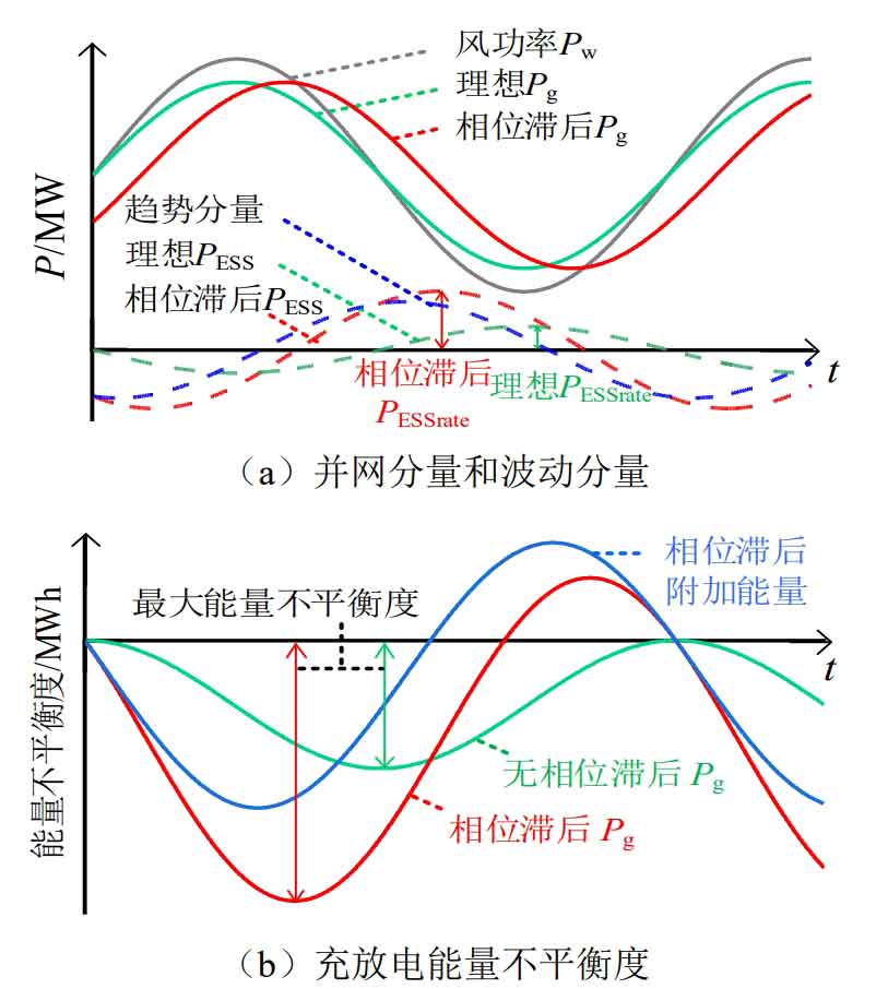
The analysis formula shows that the smoothed grid connected power phase lags behind the wind power, and as N increases, this hysteresis phenomenon becomes more severe. Based on Figure 2 (a), it can be seen that the trend component generated by phase lag is added to the reference power of battery energy storage, which increases the rated power demand and operational burden of the battery energy storage system. Meanwhile, for the dual battery integrated energy storage system, the phase lag component increases the imbalance of charge and discharge energy during the process of suppressing fluctuations in the battery energy storage system, as shown in Figure 2 (b), thereby increasing the possibility of operating in high/low SOC extreme situations in this mode, and also posing challenges to the optimization control of SOC in the battery energy storage system.
2.2 Wind power smoothing based on near zero phase adaptive filtering
2.2.1 Zero Phase Filter (ZPF)
From the formula and Figure 2, it can be seen that eliminating the phase lag of grid connected components can eliminate the additional trend components in IESS power, thereby reducing the rated power demand and operational burden of IESS. Therefore, by eliminating the phase lag term in the formula, a zero phase filter is constructed, such as the formula, which can be transformed to obtain the formula.
Substituting e ^ j · w=z into the formula can obtain the transfer function of the zero phase filter, as shown in the formula. Furthermore, by performing z-inverse transformation on the formula, the ZPF time-domain mathematical model can be obtained as follows:
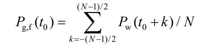
In the formula, Pg and f are the grid connected power after ZPF smoothing.
From the formula, it can be seen that the control process involves two future wind power data (N-1), and prediction technology needs to be combined to obtain the wind power for the future period. When the predicted data can accurately reflect changes in wind power, the phase difference between grid connected power and wind power is approximately zero, which is later referred to as near zero phase filter (NZPF), which can reduce the additional trend component in IESS power. Usually, only minute to several minute level wind power fluctuations need to be suppressed. Therefore, this article sets the maximum data window to 1 hour, which means the prediction interval is 30 minutes. For very few time periods with significant wind power changes, constraint intervals are used for correction. In addition, NZPF mainly utilizes the trend of wind power variation to approximately eliminate phase lag, without paying attention to local fluctuation details, and the research on prediction technology is not the focus of this article, so it will not be further elaborated.
2.2.2 Wind power smoothing based on near zero phase adaptive filtering
When the NZPF data window is fixed, smoothing can be carried out when wind power fluctuations are large to meet WPSRs. However, when wind power fluctuations are small, this control will also cause frequent input of IESS, increasing service life loss. In this regard, an adaptive NZPF is proposed, which can adaptively adjust the data window according to power fluctuations, so that the smoothing process can not only meet WPSRs, but also exit IESS operation when the fluctuations are small, reducing its losses. For very few periods with significant fluctuations in wind power, when the maximum data window is smoothed and the grid connected power still cannot meet WPSRs, a constraint interval is used for correction.
Firstly, a constraint interval model is constructed, based on the 1 minute and 10 minute time scales WPSRs, and the allowable fluctuation range of grid connected power at the current time is determined based on the historical grid connected power within the assessment time window.
The allowable fluctuation range of grid connected power for 1 minute at the current moment [P1, d (t0), P1, u (t0)] can be expressed as:
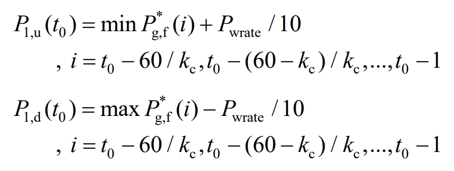
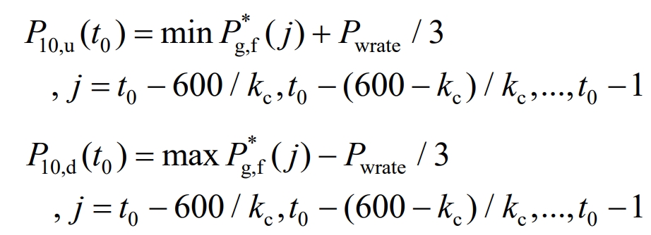
The allowable fluctuation range of grid connected power for 10 minutes at the current time [P10, d (t0), P10, u (t0)] can be expressed as:
Furthermore, the mathematical model of the grid connected power constraint interval at time t0 can be obtained as follows:
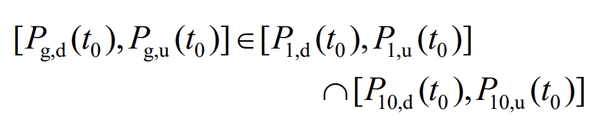
In the formula, Pg, d (t0), Pg, u (t0) are the upper and lower limits of the allowable fluctuation range of grid connected power at t0 time.
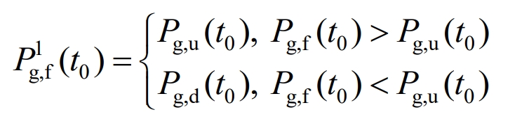
For grid connected power that still does not meet WPSRs after using maximum data window smoothing, correction shall be made according to the formula.
The power borne by IESS during this process is:
Then, a wind power smoothing process based on near zero phase adaptive filtering is proposed, as shown in Figure 3.
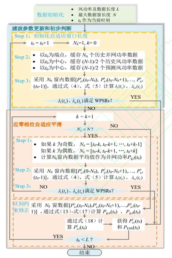
The specific execution process of the algorithm is as follows:
Step 1: Initialize the wind power data length L, with a maximum data window of N=61 minutes, and the current time being t0.
Step 2: With t0 as the center, cache (N-1)/2 historical wind power and (N-1)/2 predicted wind power. Using t0 as the endpoint, cache N0 historical grid connected power as the data basis for calculating the fluctuation rate at t0 time. The adaptive window length Nk is initialized to 1, and k is initialized to 0.
Step 3: Based on the historical grid connected power in the N0 data window, calculate the fluctuation rate of grid connected power at t0 time using the formula and determine whether it meets WPSRs. If it meets the requirements, it will be connected to the grid; If not, proceed to step 4.
Step 4: Set k=k+1 to determine whether Nk<N. If it is met, update it. When k is odd, Nk=[t0-k, t0-k+1,…, t0+k-1], and when k is even, Nk=[t0-k, t0-k+1,…, t0+k]. Calculate the average wind power within the Nk window as the grid connected power at t0, and then proceed to step 5; If not, proceed to step 6.
Step 5: Based on the grid connected power within the N0 data window, calculate the grid connected power fluctuation rate at t0 time using the formula and determine whether it meets WPSRs. If satisfied, proceed to step 7; If not, proceed to step 4.
Step 6: Calculate the constraint interval according to the formula, correct the grid connected power according to the formula, and then execute step 7.
Step 7: Determine whether the wind power is smooth, that is, whether it meets t0<L. If satisfied, smooth the end; otherwise, let t0=t0+1 and proceed to step 2.
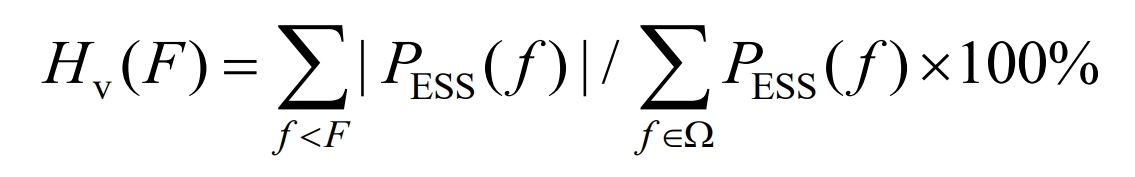
In order to evaluate the effectiveness of the strategy in this article on improving IESS output, 1) the low-frequency component content of battery energy storage system power is defined to characterize the improvement effect on phase lag and effective energy exchange of battery energy storage system. Due to phase lag, low-frequency trend components will be generated, which could have been connected to the grid and absorbed by the battery energy storage system, resulting in additional energy and life loss; 2) Maximum suppression power: As the basis for configuring the rated power of the battery energy storage system under the premise of effectively suppressing wind power fluctuations; 3) Suppression of total energy: Due to the presence of losses during the operation of the battery energy storage system, the larger this indicator, the greater the energy loss; 4) Top of running time: Evaluate the effectiveness of adaptive control strategies and adaptively exit IESS operation when the wind power is relatively stable.
1) Low frequency component content of battery energy storage system power
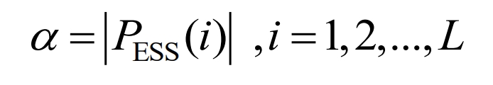
2) Maximum suppression power
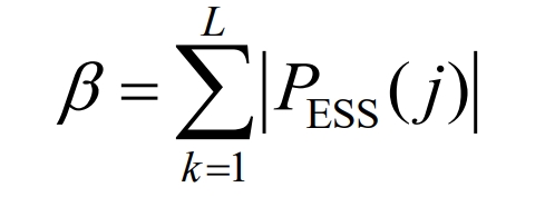
3) Suppress total energy
In the formula, F is the boundary frequency; Ω is the frequency component of the battery energy storage system power.
3. SOC optimization based on logistic dynamic interval
When using independent control of A and B batteries, the impact of frequent charging and discharging on the lifespan of energy storage batteries can be reduced. However, the capacity configuration of wind farm IESS is limited. When the total energy difference between charging and discharging is significant during the suppression process, IESS may operate in high/low SOC extreme states, which cannot effectively suppress subsequent wind power fluctuations. In this regard, equivalent SOC indicators are used to describe the overall SOC state of IESS, and they are linked to wind power smoothing. A SOC reconstruction strategy is proposed, which can dynamically adjust the charging and discharging power based on the equivalent SOC value and ensure that the adjustment process does not violate WPSRs.
3.1 Equivalent SOC indicators
When IESS is divided into A and B energy storage batteries operating independently, the SOC of the two energy storage batteries is in a decoupled state, making it impossible to evaluate the overall SOC state of IESS. Therefore, the concept of equivalent SOC is proposed, and its mathematical model is shown in the formula.
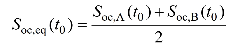
In the formula, Soc and eq are equivalent SOC of IESS; Soc, A, Soc, B refer to the SOC of A battery and B battery.
3.2 Dynamic interval adjustment based on logistic function
To ensure that WPSRs are not violated during the SOC reconstruction process, a SOC optimization strategy based on Logistic dynamic intervals is proposed. Based on the constraint interval constructed by the formula, the interval is dynamically adjusted according to the equivalent SOC value of IESS, so that the charging and discharging power adjustment is carried out within the interval, so that the adjustment process meets WPSRs.
Set adjustment rules based on equivalent SOC and real-time wind power changes, and use charging and discharging power adjustment flags to characterize, and then set adjustment functions to determine the degree of adjustment. Taking time t0 as an example, the adjustment rule is: if Soc and eq are high, it indicates that the charging group’s energy storage battery has a tendency to reach the upper limit of SOC first. To avoid operating in high SOC extreme states, power adjustment is necessary. Considering that the grid connected power obtained under this strategy has excellent wind power tracking ability under the premise of meeting WPSRs, in order to avoid violating WPSRs during the adjustment process, the power adjustment of the discharge group energy storage battery is carried out. If the wind power changes in a negative direction and reaches the discharge adjustment range at this time, the discharge power adjustment will be carried out, and the same can be obtained when Soc and eq are high. The process of adjusting the logistic dynamic interval is shown in Figure 4. The charging/discharging power adjustment flag is shown in the formula.
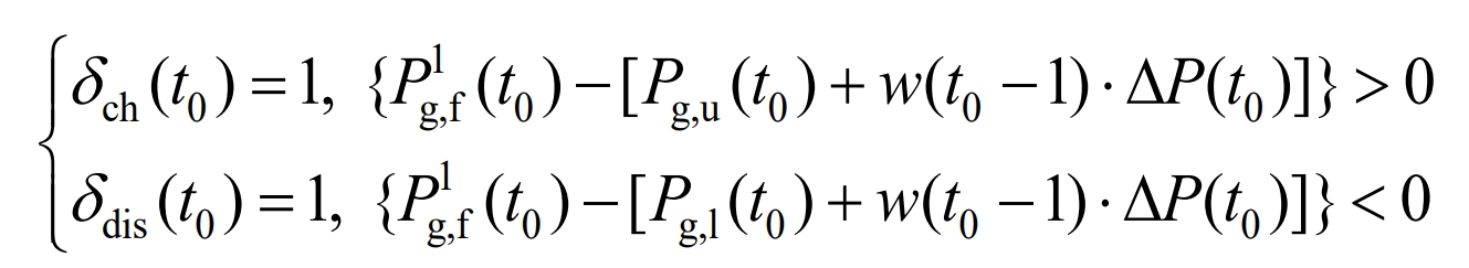
In the equation, δ Ch is the charging adjustment mark δ Dis is the discharge adjustment flag; Δ P (t) is the width of the constraint interval at time t0; W is the adjustment coefficient.
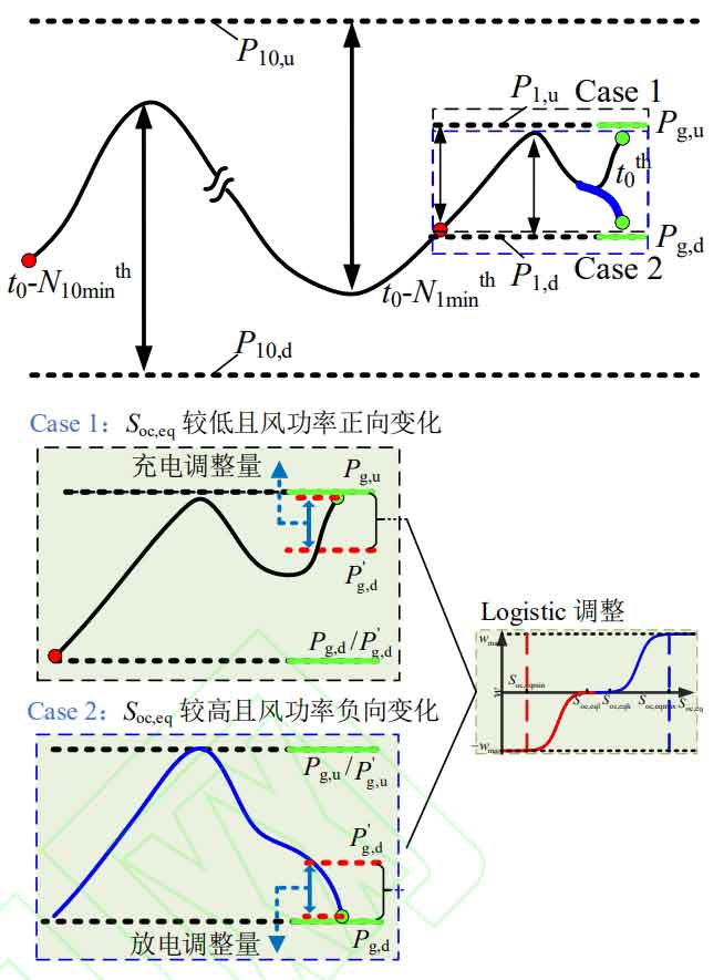
Among them, w represents the degree of adjustment of charging and discharging power, which should be determined based on the overall SOC level of IES. The basic idea is that when the IESS operates in an extreme state of high SOC, it should be adjusted to the greatest extent possible; When the overall SOC of IESS is high, dynamic adjustments are made based on the equivalent SOC value. On the basis of a series of comparative studies, the logistic function was selected as the basic form of the w-Soc, eq curve, and the function image presented an S-shape, which can achieve smooth adjustment of power. Using Soc, eq (t0) as independent variables, w as dependent variable, and adaptive factors P0 and n as parameter variables, construct a functional relationship as shown in the formula.
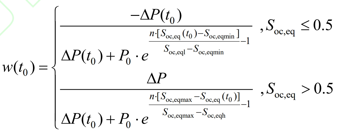
Corresponding to the formula, the adjustment curve with P0 and n as parameter variables is shown in Figure w-Soc, and the eq curve is shown in Figure 5.
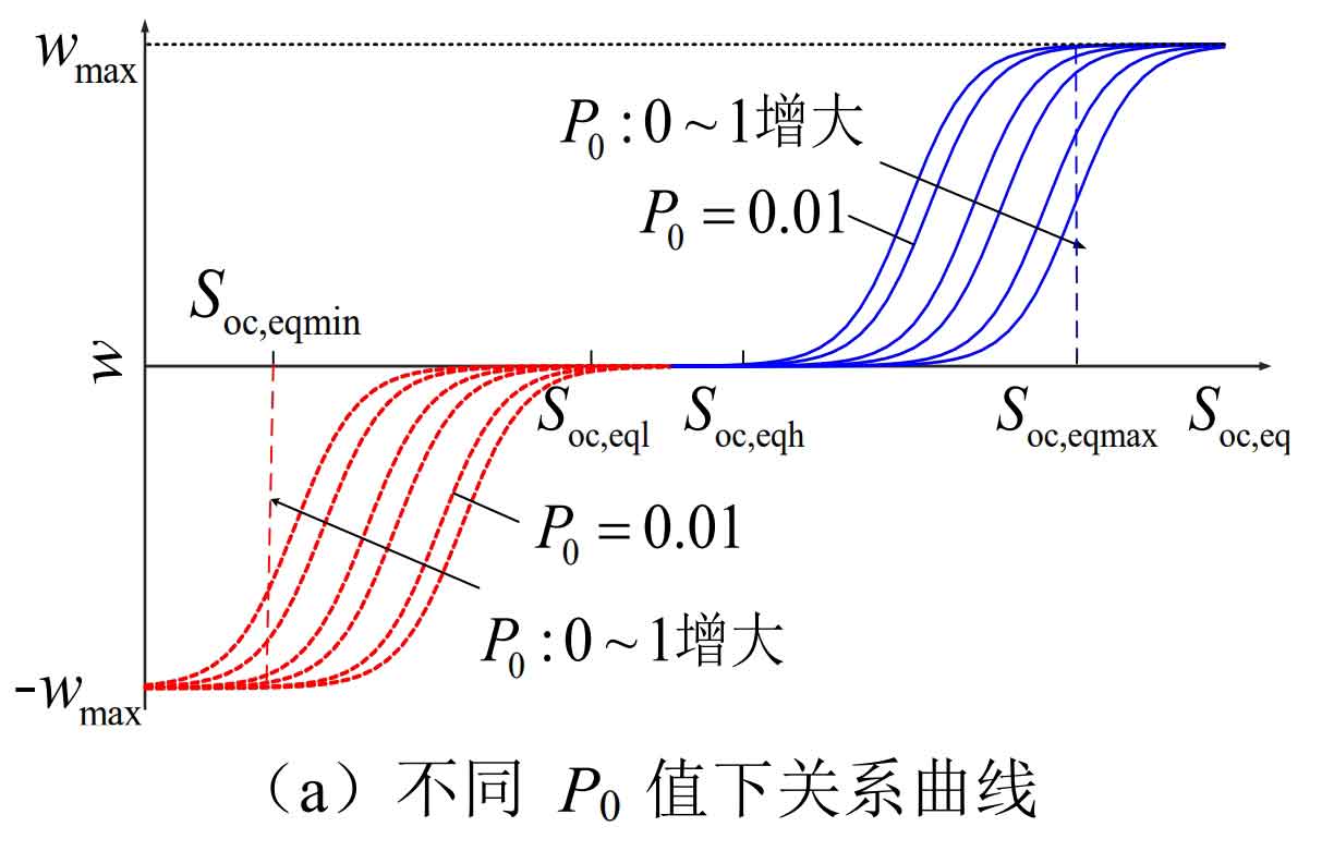
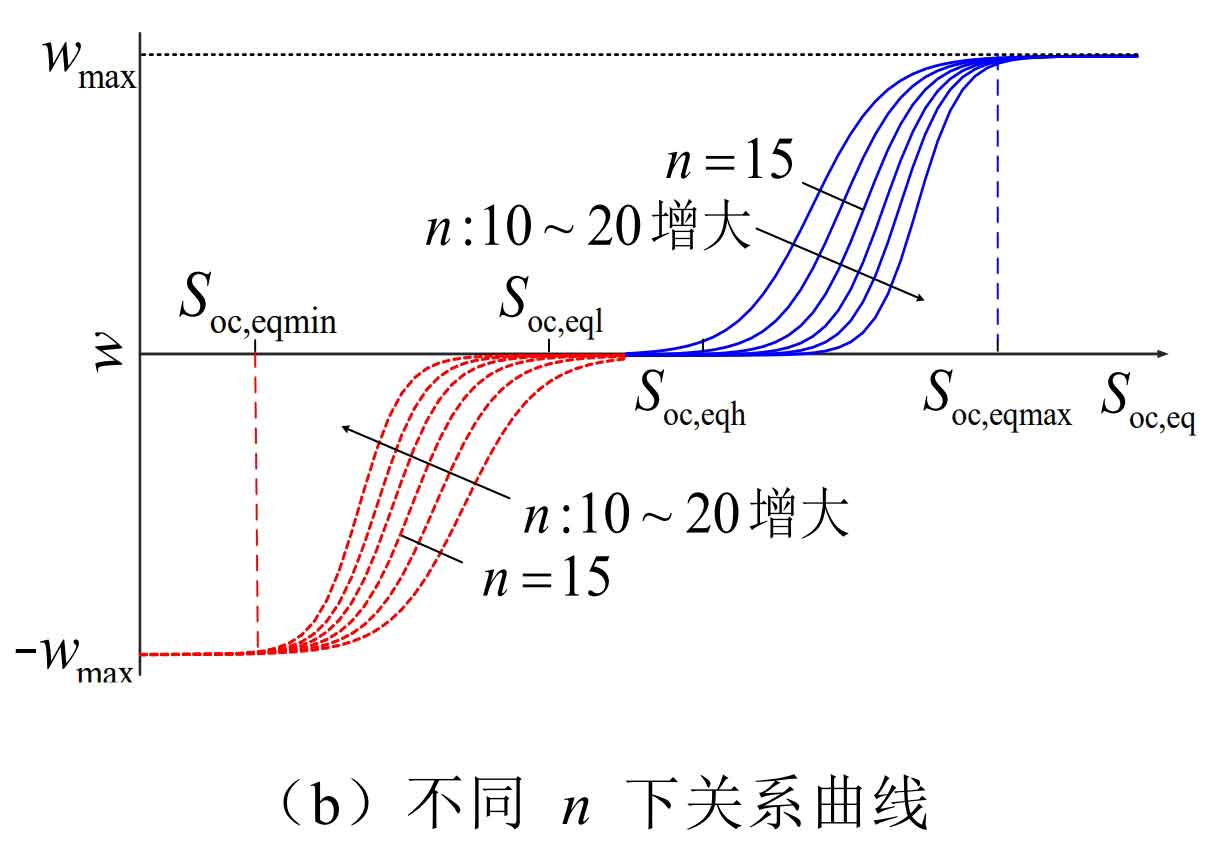
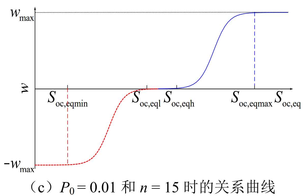
As shown in Figure 5 (a), when P0 changes in the 0-1 range, IESS is more sensitive in high/low SOC states, but can avoid frequent power adjustments when the overall SOC is good. As shown in Figure 5 (b), when n changes in the range of 10-20, IESS is more sensitive when the overall SOC is good, but has good adjustment ability in high/low SOC states. In order to balance the two, this article takes P0=0.01 and n=15, so as to have better adjustment ability under different equivalent SOC. The w-Soc, eq relationship curve is shown in Figure 5 (c).
The upper and lower limits of the adjusted interval are represented as:
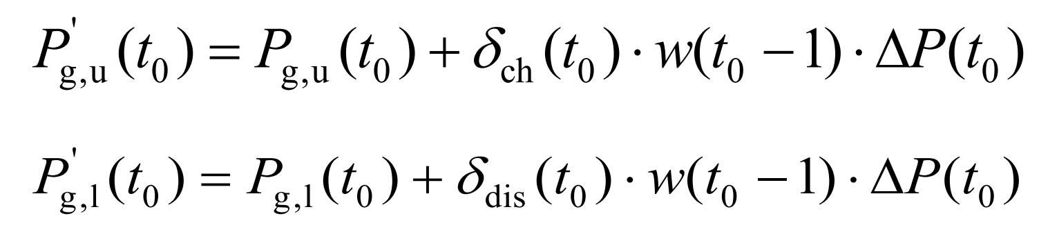
Based on the adjusted interval, the IESS power adjustment amount can be obtained as per the formula, and the adjusted IESS final power can be obtained as per the formula.
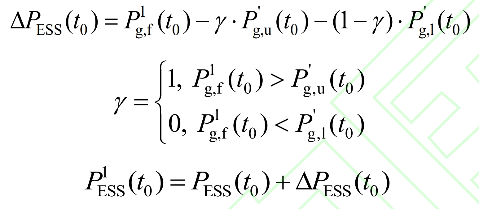
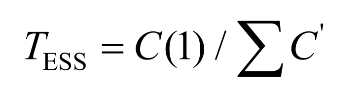
In the equation, γ = 1. 0 represents the adjustment of charging and discharging power, respectively. Furthermore, to evaluate the operating life loss of IESS, a fourth order function is first used to characterize the relationship between the number of life cycle cycles and the depth of discharge. Then, based on the rain flow counting method [25] and the equivalent cycle life method, the number of cycles C of battery energy storage at different DODs during the process of suppressing wind power fluctuations is calculated and converted to the number of cycles’ C ‘when fully charged and discharged, Then calculate the actual operating life of the battery’s energy storage based on the number of cycles C (1) during the fully charged down test.
4. Simulation analysis
Based on three scenario power data of a 50 MW wind farm with a sampling time of 1 minute, the wind power smoothing strategy based on near zero phase adaptive filtering and the battery energy storage SOC optimization strategy based on logistic dynamic interval were validated to be effective. The wind power parameters are shown in Table 1, where F *, a, F *, and max are the average and maximum fluctuation rates, respectively.
| Duration/h | F1, a (%) | F1, max (%) | F10, a (%) | F10, max (%) | |
| Scenario 1 | 24 | 3.14 | 25.33 | 14.14 | 59.25 |
| Scenario 2 | 24 | 3.82 | 21.99 | 15.74 | 47.48 |
| Scenario 3 | 96 | 3.68 | 49.62 | 15.32 | 60.82 |
4.1 Simulation analysis of wind power smoothing based on near zero phase adaptive filtering
Using wind power data from Scenario 1 and Scenario 2 as research objects, the effectiveness of this strategy is verified, and its advantages are compared with Adaptive Moving Average Filter (AMAF), Second Order High Pass Filter (SHF), and Weighted Moving Regression Filter (WMRF).
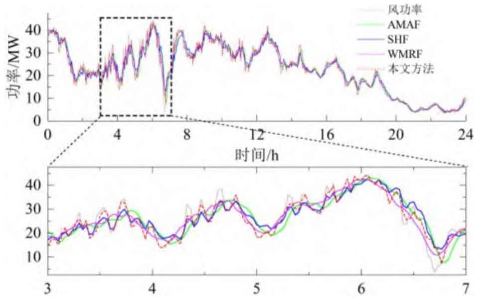
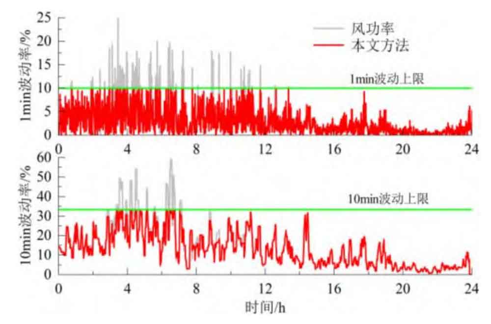
Figure 6 shows the grid connected power and volatility of AMAF, SHF, WMRF and our strategy in Scenario 1, while Figure 7 shows the adaptive window length. The optimal window length obtained using AMAF is 15. During the smoothing process, the wind power data is cached and updated based on this window length, and the average value is calculated as the grid connected power. This results in very smooth periods with small wind power fluctuations, which means that the fluctuation component borne by battery energy storage increases. In addition, during the smoothing process, due to the phase lag of the filter, the battery energy storage needs to bear additional trend components. Compared to AMAF, SHF and AMAF to some extent reduce the impact of filter phase lag. After smoothing, the grid connected power phase is close to the wind power, thereby reducing the additional low-frequency trend component borne by battery energy storage. However, when the wind power is relatively stable (such as 3 h-7 h), this control cannot adapt and adjust itself, resulting in frequent investment of the energy storage system and increasing its burden. When using this strategy, the phase of the grid connected power is close to the wind power, and it has the ability to adjust the adaptive window, effectively reducing the phase lag component and oversmooth component in the battery energy storage power, and the smoothed grid connected power meets the grid connected standard.
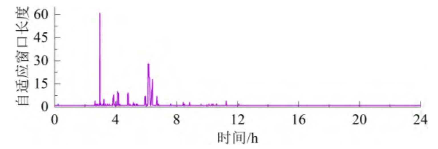
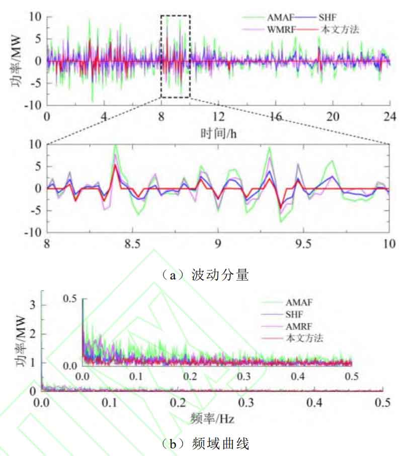
Figure 8 shows the fluctuation component borne by battery energy storage during the smoothing process. Analysis shows that the optimal window length of AMAF is determined by the maximum period of wind power fluctuation, and there is a phase lag in the grid connected power after smoothing. Therefore, the proportion of low-frequency components in the fluctuating power borne by battery energy storage is relatively large, and there is an oversmooth component; SHF and AMRF to some extent reduce the impact of controller phase lag and reduce the proportion of low-frequency components in battery energy storage power. However, when the wind power is relatively stable, due to the inability to adaptively adjust, the battery energy storage system needs to be frequently put into operation. When using this strategy, the additional components caused by the above are reduced to a certain extent, and the rated power demand for the energy storage system is minimized (according to C-rate, usually used as the basis for configuring energy storage capacity, can adaptively control the energy storage system to exit operation when the wind power is relatively stable, reducing its operational burden, and verifying the effectiveness of the strategy proposed in this paper.
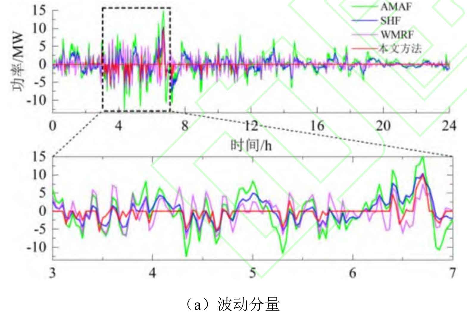
From a data perspective, as shown in Table 2, compared to AMAF, this article’s strategy α 、β And HV (0.01Hz) decreased by 37.89%, 90.27%, and 61.20%, respectively; Compared to SHF, this article’s strategy α 、β And HV (0.01Hz) decreased by 5.41%, 85.65%, and 44.14%, respectively; Compared to AMRF, this article’s strategy α 、β And HV (0.01Hz) decreased by 8.11%, 84.66%, and 47.37%, respectively; And when using this strategy, the investment time was reduced from 24 hours to 1.94 hours.
| α/MW | β/MWh | Hv(0.01Hz)/% | Top | |
| AMAF | 16.60 | 50.67 | 15.49% | 24h |
| SHF | 10.90 | 34.35 | 10.76% | 24h |
| AMRF | 11.22 | 32.13 | 11.42% | 24h |
| Strategy of article | 10.31 | 4.93 | 6.01% | 1.94h |
The grid connected components and fluctuation components obtained from scenario 2 wind power data are shown in Figure B1 and Figure B2 of Appendix B, and the relevant indicators are shown in Table B1 of Appendix B. The conclusion drawn from the analysis is consistent with Scenario 1, indicating that this strategy has good applicability in different volatility scenarios.
4.2 Optimization Simulation Analysis of Battery Energy Storage SOC
Validate the energy storage SOC optimization strategy using scenario 3 wind power data, and compare it with variable time constant first-order low-pass filtering (VTFLF) to verify its advantages. The fluctuation component is obtained by the near zero phase adaptive filtering algorithm, and its maximum smoothing power is 12.52 MW. Therefore, in the simulation, the configured energy storage system capacity is 13 MW/13 MWh, the operating SOC is 0.1-0.9, and the initial SOC value is 0.5.
(1) Analysis of SOC optimization effect
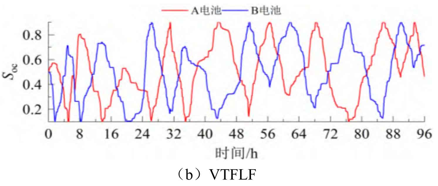
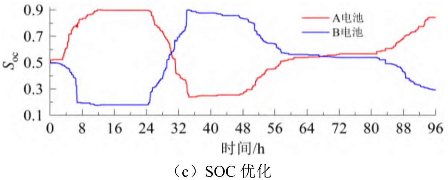
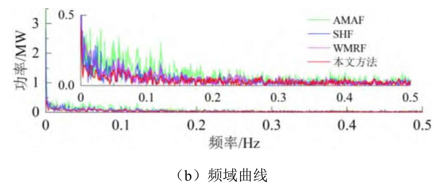
Figure 9 shows the SOC curves under SOC free optimization, VTFLF, and our strategy, while Figure 10 shows the power correction of our strategy. When there is no SOC optimization, the total charging energy continuously exceeds the total discharging energy during the operating cycle, resulting in A and B batteries being in a high SOC state when switching between charging and discharging modes for about 32 hours. Moreover, due to no power adjustment, they continue to operate in high SOC extreme states, damaging battery life and not having enough capacity to suppress subsequent positive fluctuations. When using VTFLF, although there is some improvement in SOC, due to the phase lag of the controller, the imbalance of charge and discharge energy is exacerbated to a certain extent, which increases the difficulty of control and makes the energy storage system unable to operate close to the optimal DOD during the stabilization process, with more cycles. When using this strategy, the impact of phase lag on the imbalance of charge and discharge energy is effectively reduced. At the same time, the range can be dynamically adjusted based on the equivalent SOC value, and the power can be adjusted in a timely manner to optimize the SOC, so that it can operate close to the optimal DOD, and the number of cycles can be improved.
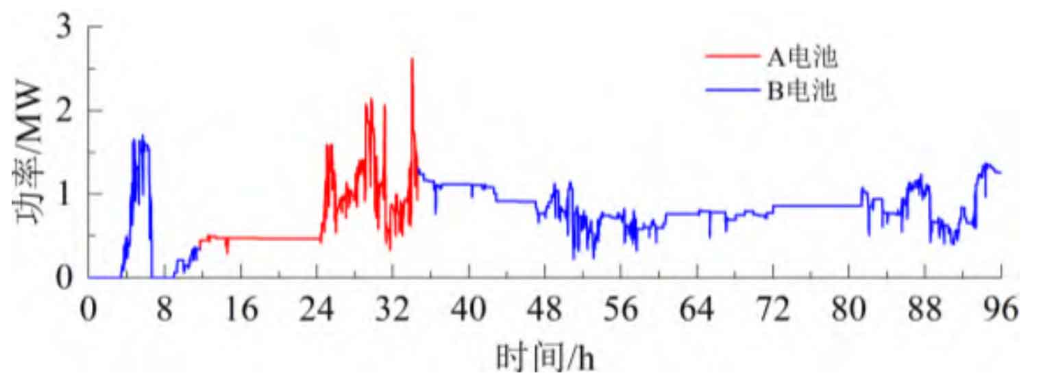
Figure 11 shows the equivalent SOC under SOC free optimization, VTFLF, and our strategy. When there is no SOC optimization, the energy storage system continues to operate at a high SOC extreme state of nearly 0.9 after 32 hours. When using VTFLF, the battery SOC is improved, but the controller phase lag makes it difficult to maintain the optimization effect of SOC in each stage. When using the strategy proposed in this article, the equivalent SOC can be controlled around 0.5, meaning that both batteries operate close to the optimal DOD, fully utilizing their cycle life.
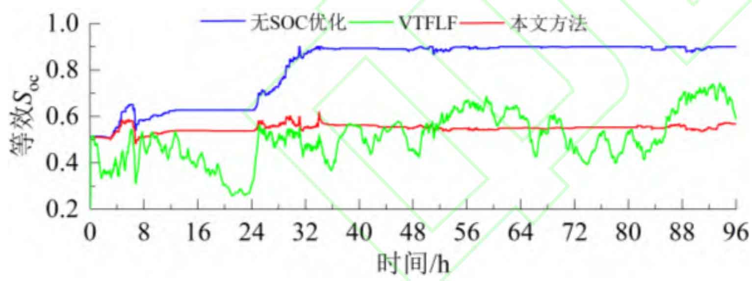
Table 3 shows the battery operating life under single battery control, VTFLF, and this article’s strategy. Due to frequent charging and discharging switching, the lifespan is greatly affected, with the shortest lifespan of 507.3 days under single battery control. When using VTFLF, the impact is reduced to some extent, but the controller has phase lag and does not have adaptive adjustment ability, which makes the battery energy storage burden large. During the flattening process, there are more cycles, and its lifespan extension effect is average, with an equivalent lifespan of 801 days. When using the strategy proposed in this article, the above problems were effectively solved, with an equivalent lifespan of 2314.4 days, which is nearly 4.6 times longer than single battery control and nearly 2.9 times longer than VTFLF, indicating good application prospects.
| A Battery Life | B battery life | Equivalent life | |
| Single battery | / | / | 507.3 |
| VTFLF | 795.3 | 806.6 | 801.0 |
| Method of article | 2311.2 | 2317.6 | 2314.4 |
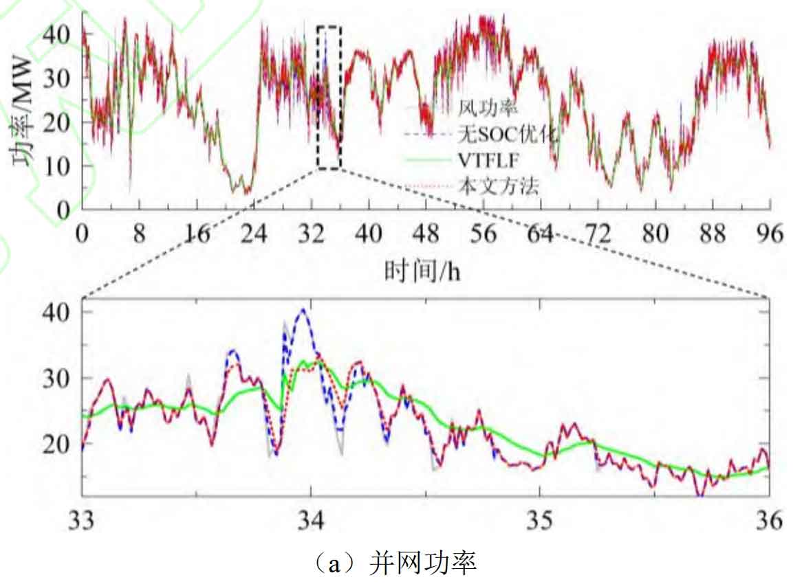
(2) Analysis of Wind Power Smoothing Effect
Figure 12 shows the grid connected power and fluctuation rate under SOC free optimization, VTFLF, and this article’s strategy. When there is no SOC optimization, due to continuous operation in high SOC extreme states, the battery’s energy storage and charging capacity is insufficient, and some periods with significant positive wind power fluctuations (such as 33 h-35 h) cannot fully respond to the reference power command. According to the formula, the actual grid connected power cannot meet the grid connection standards. When using VTFLF, the SOC state has been improved to some extent, but after smoothing, the grid connected power phase lags behind the wind power, and there is a contradiction between SOC optimization and wind power smoothing. In some periods, the grid connected power after smoothing cannot meet the requirements. When using this strategy, the phase lag problem was effectively solved and the SOC state of the battery energy storage system was maintained in good condition. Moreover, due to power adjustment within the constraint range, the actual grid connected power met the grid connected standards.
5. Conclusion
A battery integrated energy storage control strategy based on double-layer coordinated control is proposed for the scenario of wind power fluctuation smoothing. The following conclusions can be drawn through example analysis.
1) The proposed near zero phase adaptive filter smoothes the grid connected power and wind power phase to be close to the same. At the same time, it can adaptively adjust the window length based on the current power fluctuation, reducing the additional components generated by phase lag and oversmooth in the fluctuation component, thereby reducing the rated power demand and operating burden of battery energy storage.
2) The proposed optimization strategy for battery energy storage SOC based on Logistic dynamic interval can ensure that the grid connected power meets the requirements during the optimization process, and solve the extreme operating states of high/low SOC during the flattening process of the battery energy storage system. At the same time, it can enable the two batteries to operate at the optimal discharge depth, ensuring the ability to suppress subsequent wind power fluctuations and reducing battery life loss. Compared to single battery control, its lifespan is significantly extended.
Further research will be conducted in the future: 1) The impact of wind power prediction error on controller phase lag and its solutions; 2) More energy storage integration and control modes are available to improve the robustness of optimal DOD operation to energy imbalance during charging and discharging, and promote the efficient integration of energy storage systems with new energy sources.
Appendix A
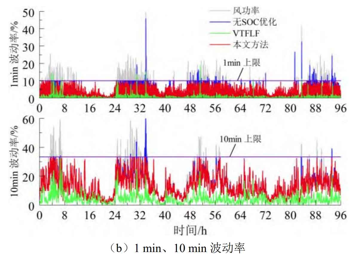
To determine the SOC range of battery energy storage operation, based on 24-hour wind power data, the fluctuation component was obtained with a sliding window of 15. Then, single battery and dual battery energy storage absorption were used respectively. By comparing the battery operating life under different DODs, the SOC range in this paper was determined with the best lifespan. Set the battery energy storage capacity to 10 MW/10 MWh, that is, both A and B batteries are 5 MW/5 MWh, and the initial SOC value of the battery is 0.5.
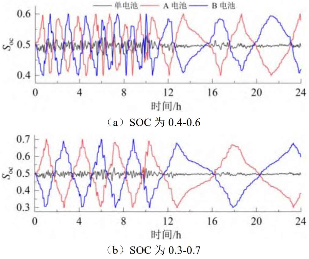
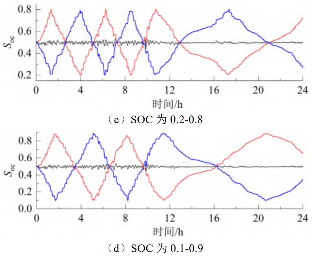
As shown in Figure A1, the SOC curves of single and dual battery energy storage under different DODs are analyzed. It can be seen that the number of charge discharge conversion times for a single battery is almost not affected by DOD, while in the dual battery mode, the number of charge discharge conversion times decreases with the increase of DOD. From Table A1, it can be seen that during the change of DOD from 0.2 to 0.8, the operating life of a single battery remained unchanged at 397.9 days, while the equivalent life of a dual battery increased from 554.8 days to 695 days. The reason for this is that although the DOD of a single battery is small, frequent charging and discharging switching leads to an increase in the number of equivalent cycles, thereby increasing the battery life loss. In addition, due to the longest battery life when DOD is set to 0.8, the SOC range for battery energy storage operation is determined to be 0.1~0.9.
| Single battery life/day | A battery life/day | B battery life/day | Equivalent battery life/day | |
| [0.4,0.6] | 397.9 | 549.2 | 560.8 | 554.8 |
| [0.3,0.7] | / | 656.4 | 604.4 | 630.4 |
| [0.2,0.8] | / | 656.4 | 604.4 | 630.4 |
| [0.1,0.9] | / | 702.8 | 687.2 | 695.0 |
Appendix B
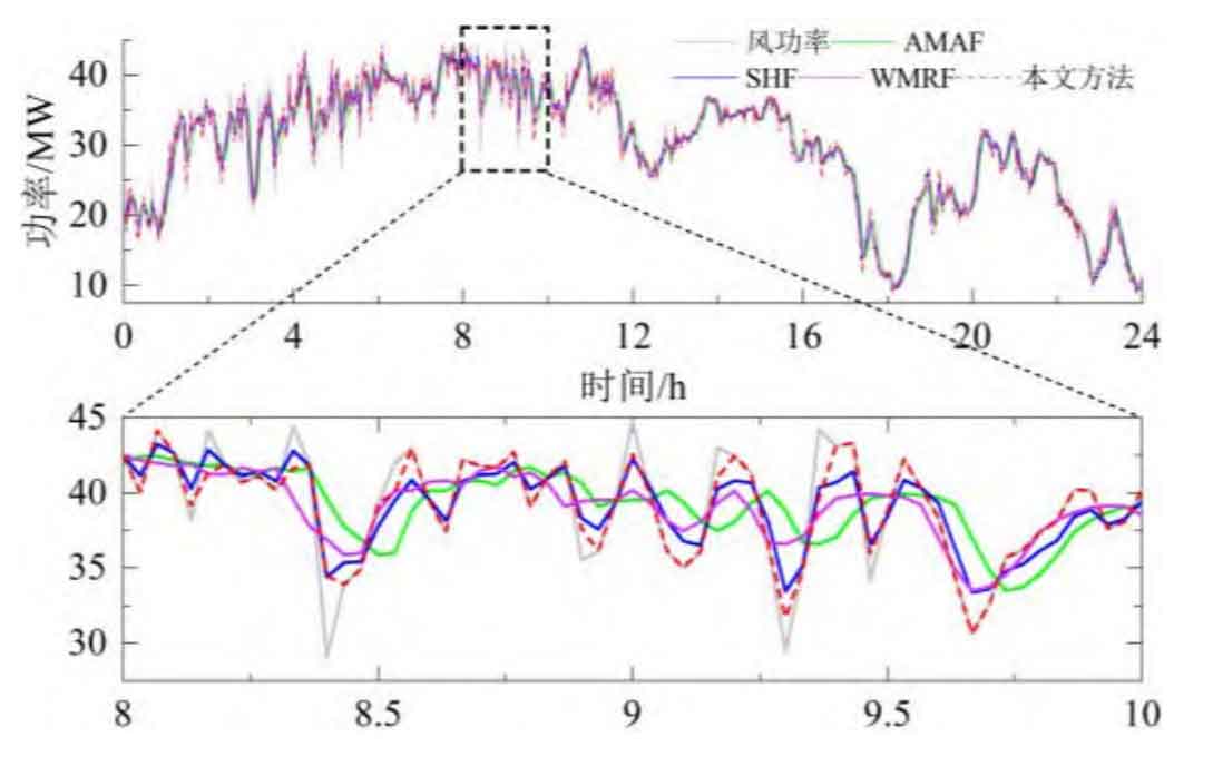
Figure B1 shows the grid connected power of scenario 2. Analysis shows that there is phase lag in the grid connected power during AMAF control. The use of SHF and WMRF effectively improves this lag situation, but it does not have adaptive adjustment ability when the wind power is relatively stable or fluctuates small. Based on Figure B2, it can be seen that it will make the battery energy storage frequently put into operation, increasing its operational burden. And this strategy effectively solves the above problems, effectively reducing the rated power demand and operational burden of the battery energy storage system. From a quantitative perspective, as shown in Table B1, compared to AMAF, this article’s strategy α、 β And HV (0.01 Hz) decreased by 48.53%, 91.55%, and 58.34%, respectively; Compared to SHF, this article’s strategy β And HV (0.01 Hz) decreased by 1.63%, 82.94%, and 43.91%, respectively; Compared to AMRF, this article’s strategy α、 β And HV (0.01 Hz) decreased by 30.78%, 87.69%, and 50.22%, respectively; When using this strategy, the duration of battery energy storage investment was reduced from 24 hours to 1.8 hours.
| α/MW | β/MWh | Hv(0.01Hz)/% | Top | |
| AMAF | 10.53 | 42.94 | 16.37% | 24h |
| SHF | 5.51 | 21.28 | 12.16% | 24h |
| AMRF | 7.83 | 29.48 | 13.7% | 24h |
| Strategy of article | 5.42 | 3.63 | 6.82% | 1.8h |