
Due to the fast charging and discharging characteristics of battery energy storage system, it is charged during low load periods and discharged during peak load periods, thereby shaving and filling the power load of isolated microgrids, alleviating the power generation pressure of microgrids during peak power consumption, ensuring the reliability of microgrid power supply, and reducing the number of start and stop times of generator units during low power consumption periods, thereby increasing the micro increase rate of power consumption of generator units. Therefore, this chapter needs to consider the charging and discharging control strategy of battery energy storage system in order to achieve good peak shaving and valley filling effects.
1. Constant power control strategy model
The constant power control strategy refers to the battery energy storage system charging and discharging at a constant power regardless of the difference between the actual power load curve and the predicted power load curve in the microgrid. The accuracy of this control strategy depends on an accurate power load prediction curve model, and the control strategy is simple with significant limitations. Figure 1 shows the charging and discharging range of battery energy storage system peak shaving and valley filling with constant power rate. This strategy is divided into the following three parts.
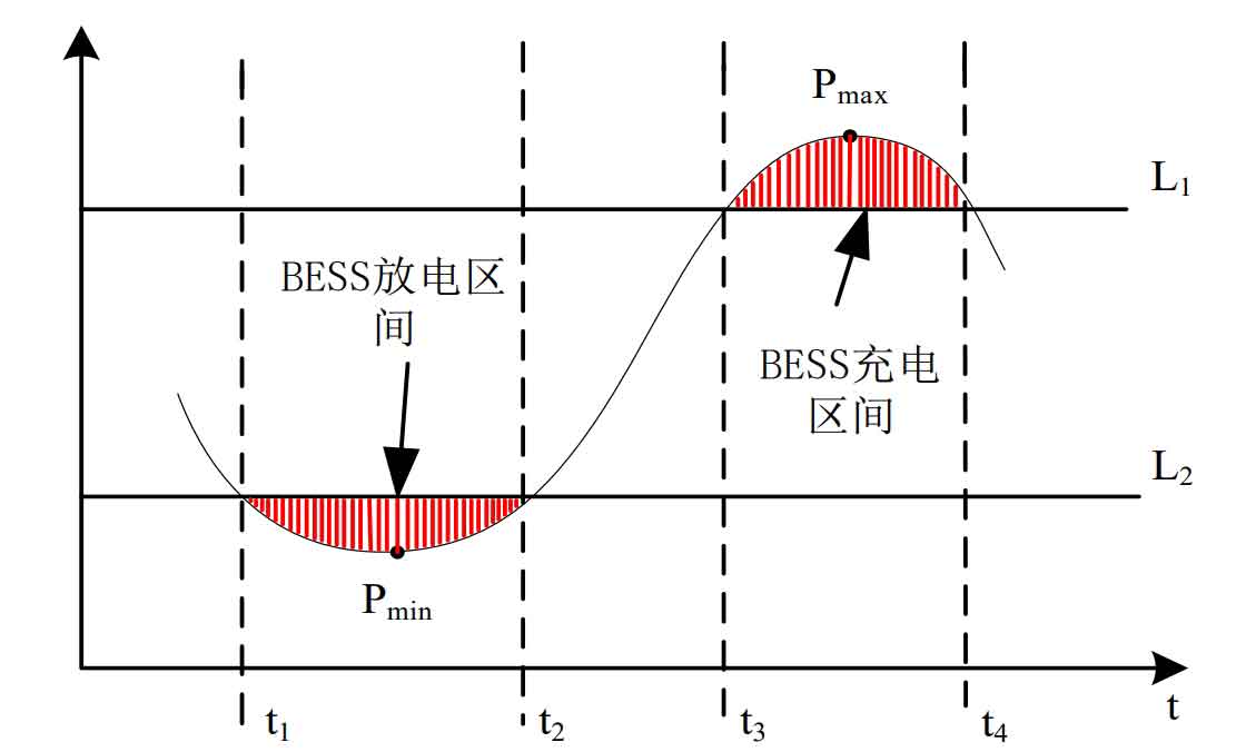
(1) Assuming the rated capacity of battery energy storage system is E and the charging and discharging power is ?. Due to the constant power charging and discharging of battery energy storage system, the charging and discharging energy of battery energy storage system is the same within the same time, so the total charging and discharging time is shown in the formula.

(2) Firstly, based on historical power load curves and other factors such as weather changes, predict the power load curve that requires constant power control strategy to control charging and discharging. Find the minimum value of power load power in the predicted power load curve (the low valley value of power load), and draw a horizontal line ? 2 parallel to the time axis t at the minimum value. Then, starting from the lowest value of the load curve, move upwards with an assumed step size ∆ M. At this point, the horizontal line ? 2 intersects with the predicted power load curve at two points, and the time interval between the two points is measured. Finally, compare the measured time interval between two points with the charging and discharging duration: if the actual measurement time interval is equal to the charging and discharging time T, then this area is the charging area; If the actual measurement time interval is not equal to the charging and discharging time T, continue to move upwards in steps ∆ M until the distance between the two is found
Determine the charging time period for battery energy storage system when the distance is equal.
(3) The determination method for battery energy storage system discharge time period and charging time period is similar. In the actual process, the predicted power load curve may have multiple peaks or valleys, and there are more than two intersections between the horizontal line and the predicted load curve. In this case, it is necessary to determine several time periods and whether they are equal to the charging and discharging time.
The charging and discharging range and power of the constant power control strategy have been determined, and the charging and discharging process still requires SOC judgment. When battery energy storage system is in the power load charging period, if ??? ≥ 0.8, then battery energy storage system is in a quiescent state, otherwise it is charged; When battery energy storage system is in the power load discharge period, if ??? ≤ 0.2, then battery energy storage system is in a static state, otherwise it is discharged; If the battery energy storage system is neither in the charging period nor the discharging period of the power load, there is no need for SOC judgment, and the battery energy storage system is in a static state.
The constant power control strategy has a simple control method and is often applied in practical engineering systems, such as Shenzhen Baoqing. However, in practical applications, the constant power control strategy excessively relies on the power load prediction curve. If the power load prediction curve deviates too much from the actual load power load curve, it is not suitable to use the constant power control strategy for charging and discharging battery energy storage system. If the constant power control strategy is used, it will greatly reduce the effect of peak shaving and valley filling. It may charge battery energy storage system during peak hours and discharge battery energy storage system during valley hours, exacerbating the peak valley difference in the microgrid, Provide negative feedback on peak shaving and valley filling effects.
2. Constant parameter power difference control strategy model
2.1 Analysis of constant parameter power difference control strategy
Battery energy storage system may have multiple limiting factors during charging and discharging, but the constant power charging and discharging control strategy does not consider these factors and excessively relies on the accuracy of power load curve prediction. The constant parameter power difference control strategy mainly considers the capacity and power of battery energy storage system to avoid the above problems. In addition, the battery energy storage system life model was also considered, specifying the charging frequency of the battery energy storage system. In the power difference control strategy, the daily average load power ??? is calculated based on the predicted power load curve, and ??? is obtained. ?1 and ?2 are then compared with the predicted power load curve to obtain the charging and discharging power of battery energy storage system in the next time period, as shown in the formula.
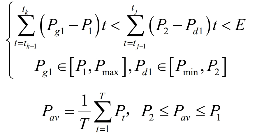
In the formula, ??1 and ??1 are the loads during the peak and low load periods, respectively; ? 1 is the lower limit value of battery energy storage system discharge power; ? 2 is the upper limit value of battery energy storage system charging power; ????, ??? are the peak and valley values of the load; ??? is the average daily load power; ∆ ? represents unit time.
The specific steps of the constant parameter power difference control strategy are as follows.
Step 1: Calculate the average value ??? based on the predicted daily load curve, and determine the initial values of ?1 and ?2.
Step 2: Iteration with an initial value of ??? and a step size of ∆? until the battery energy storage system total charge and discharge amounts are approximately equal.
Step 3: Determine the upper charging limit value ? 2 and lower discharging limit value ? 1 of battery energy storage system according to Step 2, and determine the charging and discharging power according to the actual situation.
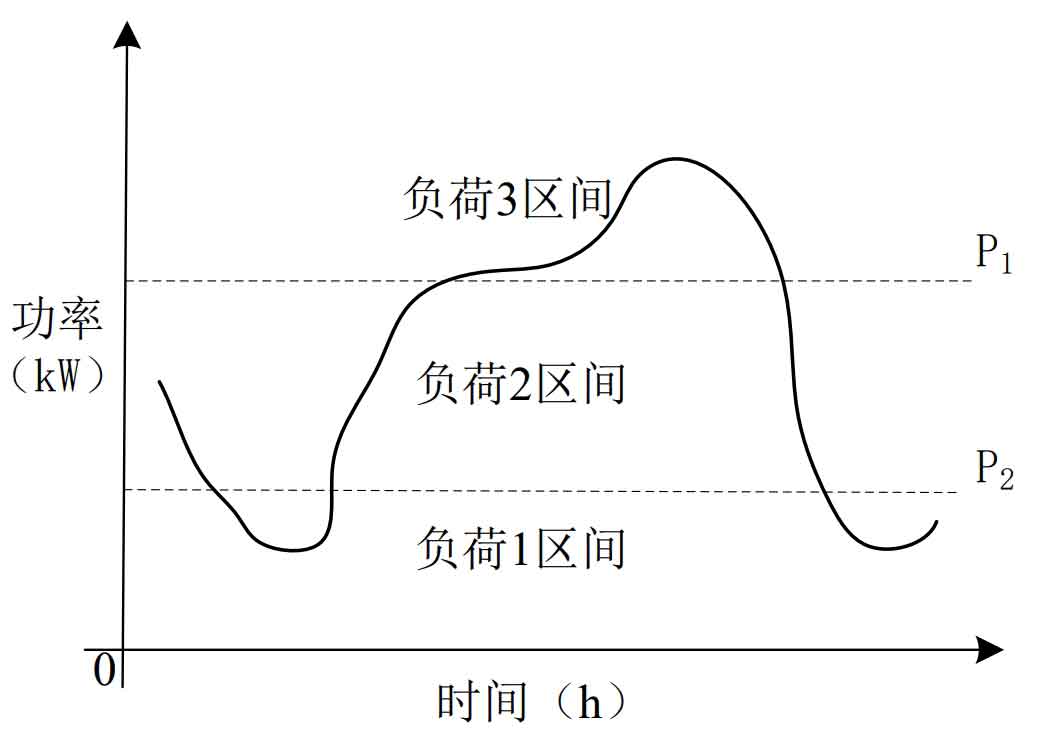
From Figure 2, it can be seen that the load is divided into three parts based on ? 1 and ? 2, which are respectively load 1 interval, load 2 interval, and load 3 interval.
(1) Load range 1, Battery energy storage system charging, with a charging power of ??, as shown in the formula.
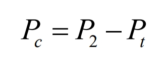
In the formula, ?? is the battery energy storage system charging power, and ?? is the actual power of the power load at time t.
(2) Load range 2, with battery energy storage system stationary (battery energy storage system neither charges nor discharges) as shown in the formula.
In the formula, ?? is the battery energy storage system discharge power.
(3) Load range 3, discharge power ??, as shown in the formula.
2.2 Objective function
In a microgrid operating on isolated islands, the main role of battery energy storage system is to perform peak shaving and valley filling of power loads. During the peak of power load, battery energy storage system acts as a power source to supply power to power equipment, achieving the goal of reducing the peak of power load. During the valley of power load, battery energy storage system acts as a load, consuming the power generation of the microgrid, achieving the goal of increasing the valley of power load, and thus achieving the goal of peak shaving and valley filling of the microgrid. The standard deviation D of power load is used as an indicator to evaluate the effect of peak shaving and valley filling. The smaller ?, the better the effect of peak shaving and valley filling. The expression is shown in the formula.
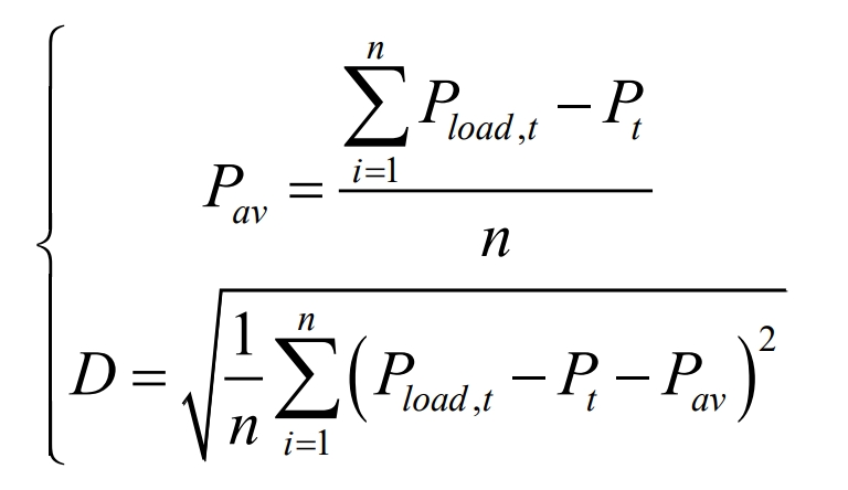
In the formula: ?????, ? is the power of the load at the moment before peak shaving and valley filling; ?? is the charging and discharging power of battery energy storage system, and when ??>0, battery energy storage system discharges; Charge battery energy storage system when ??<0; When ??=0, leave the battery energy storage system stationary.
2.3 Constraints
In the battery energy storage system optimization control model of island operating microgrids, only the physical models related to battery energy storage system and the constraints generated by power balance of the grid are considered.
(1) Power balance constraints of the power grid:
In the formula: ???? is the output power of the power grid; ????? is the load power of the user; ???? is the output of the energy storage battery. When the energy storage battery is discharged, ????>0, otherwise, Pess ≤ 0.
(2) Constraints of SOC
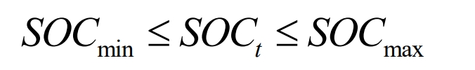
In the formula, ????? is the minimum SOC value of battery energy storage system; ?????? is the maximum SOC value of battery energy storage system, where SOCmin=20%; SOCmax=80%.
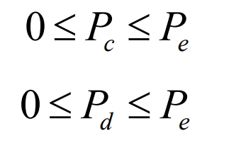
(3) battery energy storage system charging and discharging power constraints
2.4 Objective function evaluation indicators
A study on the control strategy of battery energy storage system peak shaving and valley filling charging and discharging in microgrids under islanded operation was conducted. Four mathematical equations were used to evaluate the effect of peak shaving and valley filling, including peak valley difference, peak valley coefficient, peak valley difference rate, and standard deviation of power load fluctuation.
(1) Peak valley difference
In the formula, ???? is the peak value of the power load wave; ??? is the valley value of the power load; ∆ ? Absolute peak valley value of power load, indicating the difference between peak and valley of power load at a certain time scale. The smaller ∆?, the smaller the maximum deviation value of power load.
(2) Peak valley coefficient
In the formula, ? is the coefficient of peak valley difference of power load, representing the flatness of the power load curve at a certain time scale. If ? is small, the load curve becomes steeper and the peak valley difference becomes larger.
(3) Peak valley difference
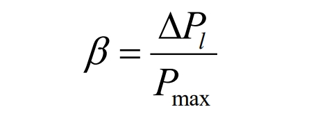
In the formula, ? is the peak valley difference rate of power load, indicating the degree of power load fluctuation at a certain time scale. The smaller ?, the smaller the range of power load fluctuation.
(4) Standard deviation of power load fluctuation
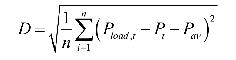
In the formula, ? is the standard deviation of power load fluctuation, indicating the degree of dispersion of power load at a certain time scale. The smaller ?, the smaller the degree of dispersion of load; ? is the period during which the power load curve is sampled.
3. Optimization of Charge and Discharge Control Strategy Based on Improved Particle Swarm Optimization Algorithm
The ABC algorithm has no memory and is easy to operate. The improved ABC algorithm has good convergence; Particle Swarm Optimization (PSO) has memory, complex operations, and poor convergence; The capacity configuration of battery energy storage system does not require historical data, while the constant parameter power difference control strategy requires historical data; So, the improved ABC algorithm is used to configure the capacity of battery energy storage system, and the improved particle swarm optimization algorithm is used to optimize the constant parameter power difference control strategy.
3.1 Analysis of Particle Swarm Optimization Algorithm
Since the 1930s, computer scientists have been conducting simulation research on natural organisms. They have observed that applying evolution and natural selection in the biological world to computer algorithms can simplify algorithm processes and optimize algorithm solving efficiency. PSO, jointly proposed by Dr. Eberhart and Dr. Kennedy in 1995, is an artificial intelligence algorithm that allows bird groups to determine the distance between their location and food within a certain space, even if they do not know the specific location of the food. Through information exchange between birds, the bird group can search for food in the same area at a certain speed and ultimately obtain food. The predatory behavior of bird flocks is very similar to the problem of finding the optimal solution when solving algorithms. The PSO algorithm evolved from the characteristic behavior of bird populations during predation mentioned above. Equivalent modeling of bird predation behavior, treating each bird as a particle in a D-dimensional solution space. All particles are deployed in this D-dimensional search space, and each particle has its own position information in the space. The position of each particle can represent the distance between the bird and the food. The position information of the particles is substituted into the fitness function, When the fitness function value is smaller, it indicates that the particle’s position in space is better. Through a limited number of iterations, the particle’s position information is updated, and each iteration of the particle’s position will change accordingly. When the iteration number ends, the output is the optimal solution found by the algorithm. This algorithm is an iterative optimization tool that can achieve global search in solving complex problems, improving the speed and accuracy of seeking the optimal solution. It has been widely used in fields such as function solving and image processing. Reynolds discovered a pattern in studying bird flight, where seemingly complex bird groups are actually generated by the interaction and communication between each bird. That is, each particle cooperates and competes with each other, and gradually approaches the optimal solution until it converges at the optimal solution in the global space.
Update the velocity and position of particles according to the following formula, as shown in the formula.
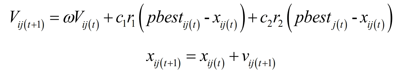
In the formula, i represents the i-th particle number; J is the jth dimension of the particle; ω Is the inertia factor; C1 and c2 are learning factors; Vij (t+1) is the component of particle i’s velocity in the jth dimension when it evolves to t+1 generation; Vij (t) is the component of particle i’s velocity in the jth dimension when it evolves to generation t; Pbestij (t) is the optimal position component of particle i evolving to the jth dimensional individual of generation t; Gbestij (t) is the optimal position component of the entire particle swarm from particle i to the jth dimension of generation t; Xij (t+1) is the component of particle i at the jth dimensional position during evolution to t+1 generation; Xij (t) is the component of particle i at the jth dimensional position during its evolution to generation t.
The steps of particle swarm optimization algorithm are as follows
Step 1: Set basic particle swarm parameters, such as the number of particles, inertia weight coefficients, particle dimensions, upper and lower limits for each particle dimension, acceleration factor values, maximum iteration times, etc.
Step 2: Randomly initialize the speed and position of particles generated in the space, and set the initial individual optimal position of each particle, and compare to obtain the initial global optimal particle position.
Step 3: Use the formula velocity equation and formula position equation to update the position and velocity of particles.
Step 4: Compare with the initial optimal position of the particles, and if the updated optimal position of the particles is better than the initial optimal position of the particles, replace it with the individual optimal position.
Step 5: Through Step 4, the individual optimal positions of all particles will be obtained. After comparing with the current global optimal position, the updated global optimal position will be obtained.
Step 6: Determine whether the number of iterations has reached the maximum number of iterations set by the algorithm. If not, return to step 3. If it has, the algorithm ends and outputs the result.
3.2 Particle Swarm Optimization and Objective Function Solving Process
The particle swarm optimization algorithm still has the problem of easily falling into local optima, and the ergodicity of chaos theory is used to solve the local optimization problem of the particle swarm algorithm. Because chaos theory has ergodicity and can effectively change the distribution of particles, it improves the global search ability of the algorithm. The classic chaotic system is a Logistic map, as shown in the formula.
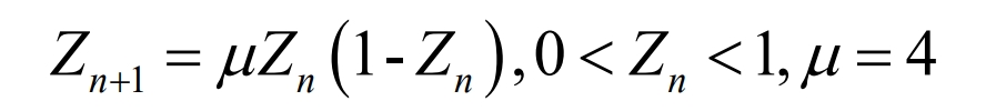
In the formula, ??+1 represents the next state of the chaotic system; ?? is the current state of the chaotic system; ?=4 is a completely chaotic state.
The specific steps of the algorithm are as follows and the algorithm flowchart.
Step 1: Initialization: Set the number of particles (num=60), particle dimension (D=3), learning factor (c1=c2=2), and inertia factor( ω = 0.9), particle velocity, maximum number of iterations, particle accuracy, initialization of chaotic variables, excluding the 5 fixed points (0,0.25, 0.5, 0.75) in the chaotic iteration equation.
Step 2: When t=0, generate D chaotic variable factors chaos (i), where 1 ≤ i ≤ D and t is the number of iterations.
Step 3: Calculate the fitness value of particles and update their velocity and position based on the formula.
Step 4: Determine whether the particle is trapped in a local optimum (based on the proximity or coincidence of multiple particle positions). If it is not a local optimum, proceed to step 6, otherwise proceed to the next step.
Step 5: Use chaotic variables to assign chaotic values to particle positions, and substitute them into the Logistic map. As shown in the formula, iteratively distinguish between the chaotic variable intervals [0,1] and map the corresponding variable value intervals.
Step 6: Determine the solution gbest and pbest for particle multi-objective fitness.
Step 7: Determine whether the particle meets the termination condition. If it does not meet the termination condition, proceed to Step 3, otherwise proceed to the next step.
Step 8: Output the result and the program ends.
The solution process of the objective function.
Step 1: Determine the load range for battery energy storage system charging and discharging based on the daily power load curve.
Step 2: Determine whether battery energy storage system is overcharged or discharged. If not, proceed to step four; If so, proceed to step three.
Step 3: Use an improved particle swarm optimization algorithm to redefine the load interval.
Step 4: Determine the charging and discharging power to charge and discharge battery energy storage system.
Step 5: Determine whether the time requirement is met. If not, return to Step 2. If so, end.
4. Simulation Results and Analysis
Taking the battery energy storage system peak shaving and valley filling of a certain island operating microgrid as an example for simulation, the maximum power load power of the island operating microgrid is 4050kW, the minimum power load power is 1550 kW, and the peak valley difference is 2500. As shown in the figure, the energy storage battery in the battery energy storage system in the microgrid is a lithium-ion battery, with a rated power of 900kW, a maximum charging power of 600kW, and a minimum charging power of 600kW. The SOC range is [0.2, 0.8]. The simulation results verify the effect of peak shaving and valley filling of microgrid power load under constant power control strategy and constant parameter power difference control strategy, as well as the power load situation of microgrid under constant parameter power difference control strategy using pre improved PSO and post improved PSO solutions. In order to simplify the solving process of the algorithm, new energy generation is equivalent to the load side.
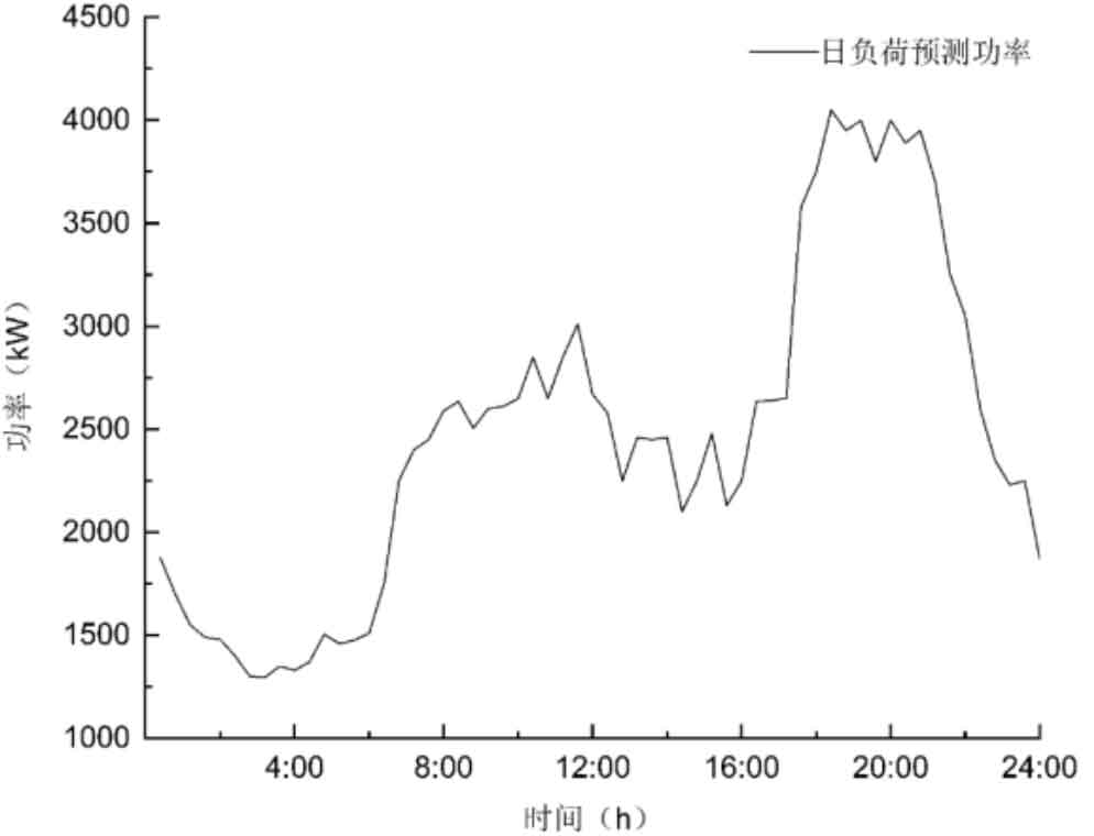
Figure 3 shows the daily load prediction curve of the island operating microgrid. The power load is during the low valley period from 2:00 to 4:00 and the peak period from 18:00 to 23:30, which is basically consistent with the actual situation.
| Parameter Name | Data |
| Rated capacity (kWh) | 900 |
| Maximum charging power (kW) | 600 |
| Maximum discharge power (kW) | 600 |
| Maximum SOC (%) | 80 |
| Minimum SOC (%) | 20 |
4.1 Simulation of constant power control strategy
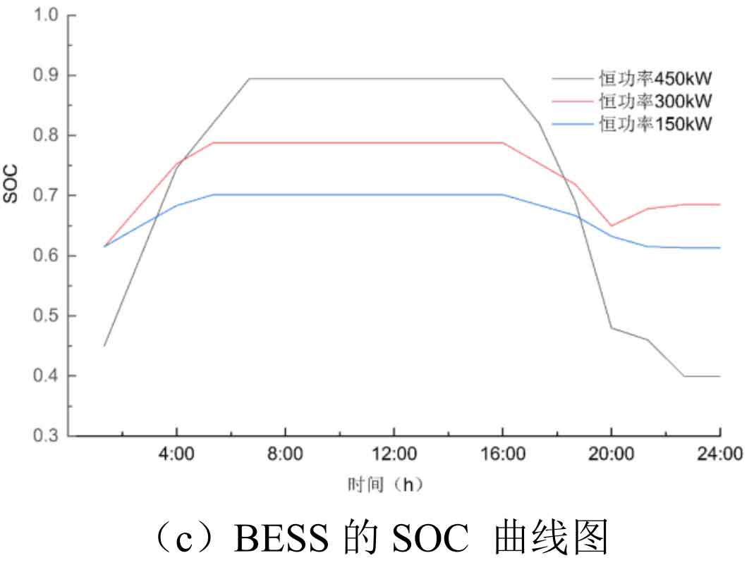
Under the constant power control strategy, the charging and discharging powers of battery energy storage system are set to 450kW, 300kW, and 150kW respectively for charging and discharging. When the power load is low, battery energy storage system charges; During peak power load, battery energy storage system discharges; To achieve the goal of battery energy storage system peak shaving and valley filling, the simulation diagram is shown in Figure 4.
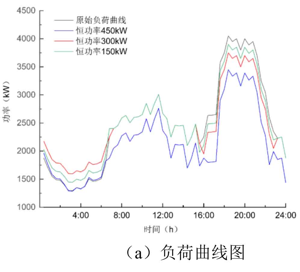
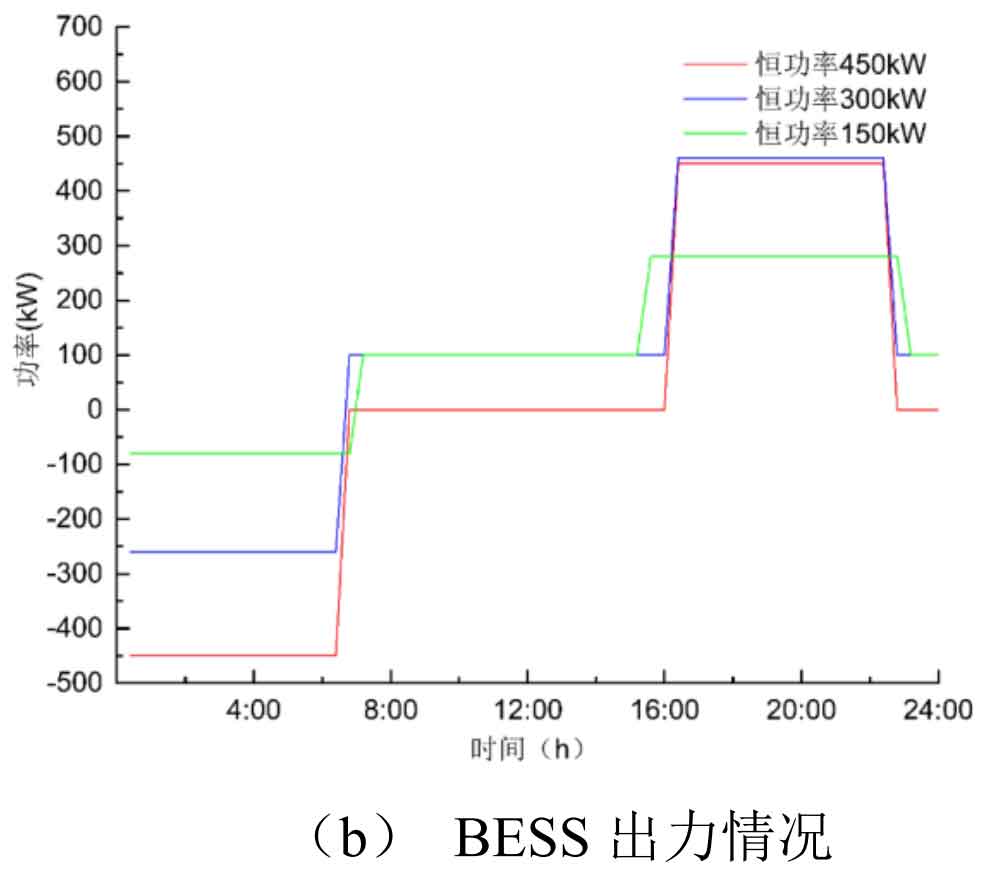
As shown in Figure 4, setting different charging and discharging powers has different effects on the load curve. When controlled at a constant power of 150kW, the curve shrinks slowly compared to the original load curve, because the power set by battery energy storage system is smaller, but it can be charged and discharged for a long time. When controlled at a constant power of 450kW, the curve decreases significantly compared to the original curve at peak and rises significantly at valley, achieving the effect of peak shaving and valley filling. However, the curve set in this situation will experience significant load fluctuations from 18:00 to 21:00, bringing a significant impact on the power fluctuation of the microgrid. When controlled at a constant power of 300kW, peak shaving and valley filling can also achieve good results, However, there will also be significant load jumping when decomposing the line.
In summary, taking into account the output situation of battery energy storage system and the peak shaving and valley filling situation, both 450kW constant power control and 300kW constant power control can achieve good peak shaving and valley filling effects. However, simulation has found that this control strategy has certain problems in battery energy storage system setting, with excessive power and sudden changes in the load curve at the boundary, and the charging and discharging time is too long when the setting is too small; Moreover, under constant power control of 450kW, battery energy storage system may experience overcharging and discharging issues. In this case, a constant parameter power difference control strategy appears.
4.2 Simulation of Constant Parameter Power Difference Control Strategy
Based on the case in Figure 3, the typical daily load curve shows an average daily load power of ???=2469.08 ??. Set the iteration step ∆ ?=1 ??, calculate the lower discharge power ? 1=3255.08 ?? of battery energy storage system, and the upper charging power ? 2=2129.17 ??. Use a constant parameter power difference control strategy for simulation, and the simulation results are shown in Figure 5.
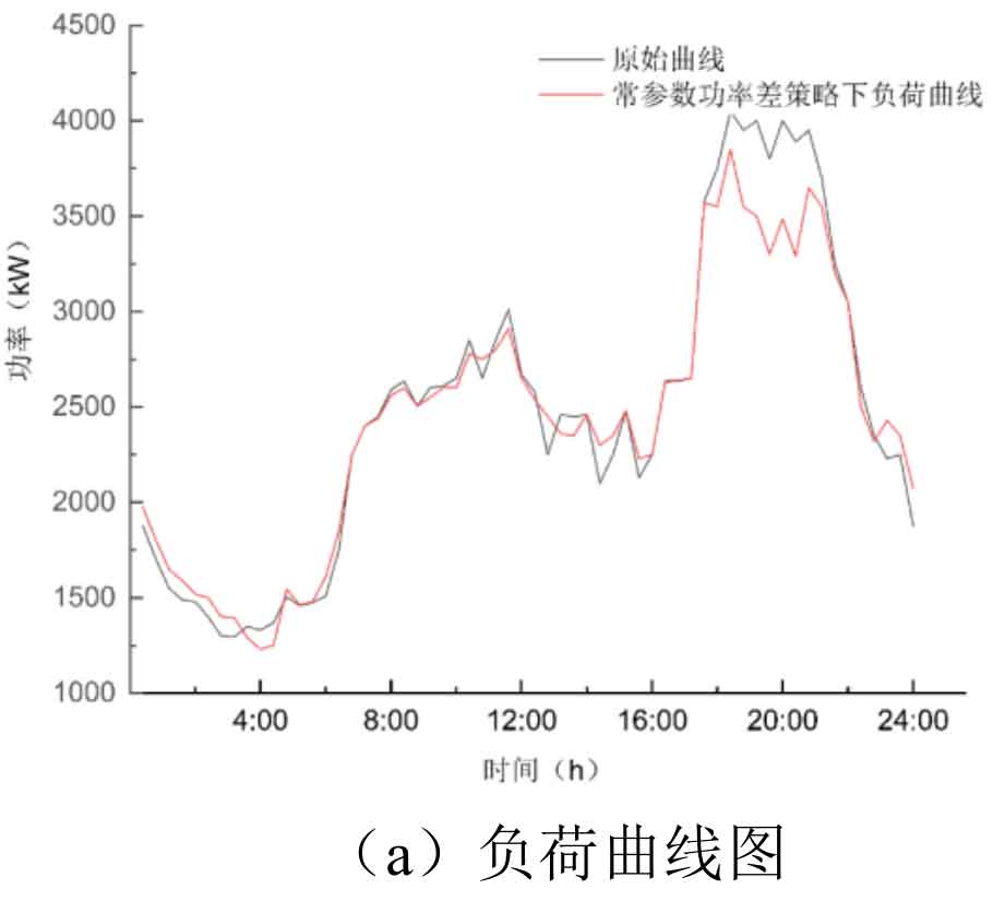
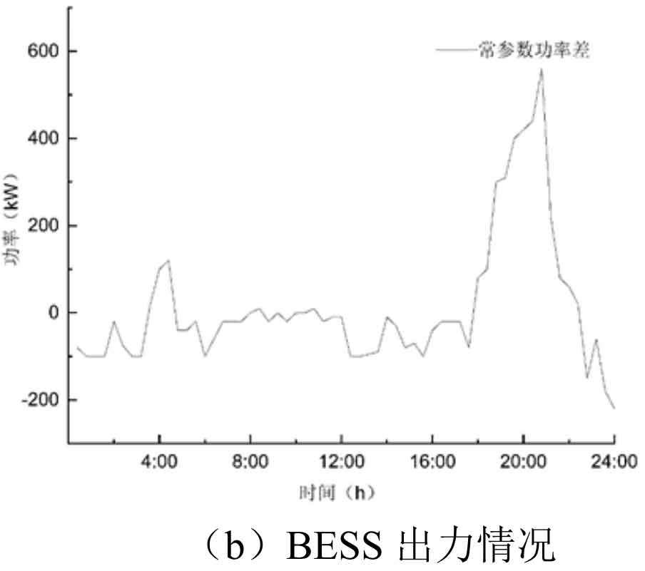
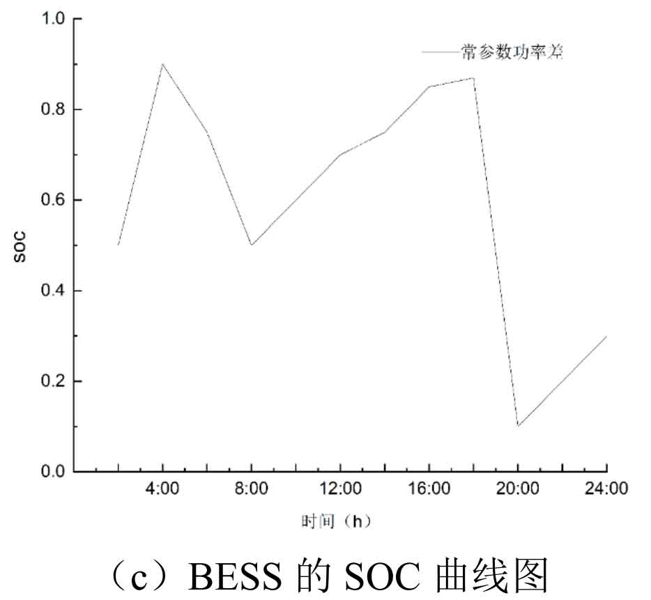
As shown in Figure 5, under the constant parameter power difference control strategy, the peak shaving and valley filling effect can be achieved effectively, and the system shows obvious performance around 4:00 and 20:00. The constant parameter book power difference control strategy has a relatively accurate effect on the peak valley difference of the load curve, without significant load jump, improving the quality of power grid operation. However, around 4:00, under the constant parameter power difference control strategy, the power of the power load reaches its lowest point, and there is a phenomenon of overcharging and discharging of the SOC value of battery energy storage system around 4:00 and 18:00, which is caused by the local optimization problem when using particle swarm optimization algorithm to solve the objective function.
The comparison between constant power control strategy and constant parameter control strategy is as follows:
(1) The constant power control strategy has a simple control method and is often applied in practical engineering systems. However, in practical applications, the constant power control strategy excessively relies on the power load prediction curve. If the charging and discharging power of the constant power control strategy is set too high, it will cause a jump in the power load curve; Setting the charging and discharging power too low will prolong the charging and discharging time of battery energy storage system, which is not economical.
(2) The constant parameter power difference control strategy is more complex than the constant power control strategy. In practical applications, the constant parameter power difference control strategy has lower requirements for the power load prediction model, and the power load curve is smoother after peak shaving and valley filling, without any load jumping.
(3) In practical applications, both control strategies have certain effects on peak shaving and valley filling of power loads. The constant parameter power difference control strategy is superior to the constant power control strategy, and there is no load jump, significantly reducing the phenomenon of battery energy storage system overcharging and discharging.
4.3 Simulation of Improved Particle Swarm Optimization Algorithm with Constant Parameter Power Difference Control Strategy
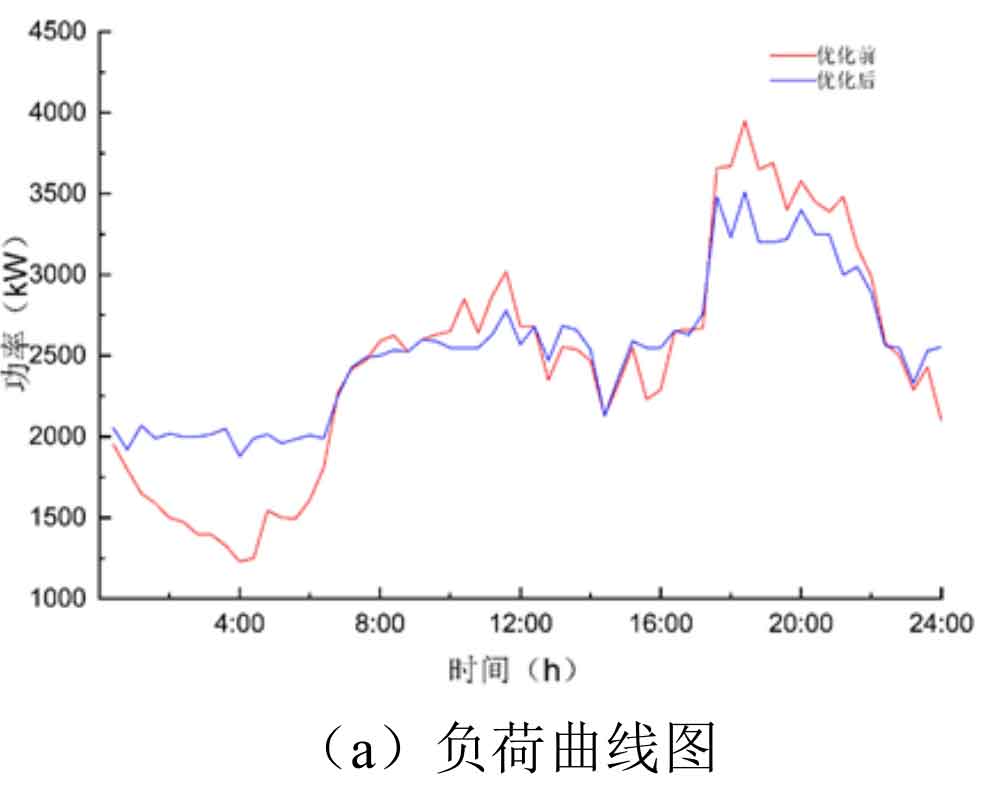
From Figure 6 (a), it can be seen that the load curve of the control strategy before optimization is relatively steep. After optimization, the control strategy significantly improves the load curve and becomes smoother, thereby reducing the peak valley difference of the load and improving the smoothness of the load curve, achieving the goal of peak shaving and valley filling. Table shows that the peak load has decreased from 4050kW under the constant parameter control strategy to 3400kW under the pre optimization control strategy; The load valley value has increased from 1295kW under the constant parameter control strategy to 1895kW under the optimized differential control strategy; The standard deviation of the load decreased by 25.07% from 802.31 under the pre optimization control strategy to 601.14 under the post optimization control strategy, and the average value of the load decreased from 2469.18kW under the pre optimization control strategy to 2522.20kW under the post optimization control strategy.
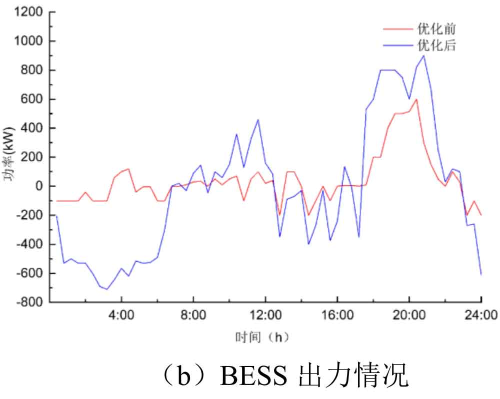
From Figure 6 (b), it can be seen that the output state of battery energy storage system changes with the change of load power. Before optimization, the output of the battery energy storage system is relatively flat under the control strategy, while after optimization, the output fluctuation of battery energy storage system is large under the control strategy. Therefore, the effect of load peak shaving and valley filling is ensured, the output of the generator set is reduced, and the economic efficiency of the power grid is improved.
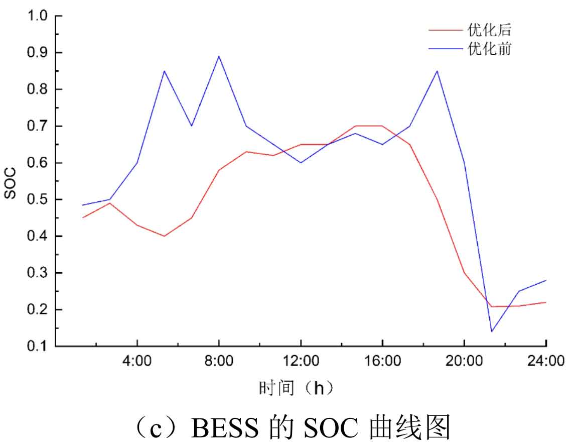
From Figure 6 (c), it can be seen that the SOC of the control strategy before optimization was too high or too low, while the SOC range of the battery energy storage system fluctuated between [0.2,0.8] under the action of the optimized control strategy. This solves the problem of overcharging and discharging of the battery energy storage system, which is beneficial for extending the service life of the battery energy storage system.
| Before optimization | After optimization | Absolute values of two control strategies | Absolute values of two control strategies | |
| Peak value (kW) | 4030 | 3400 | 630 | 15.63% |
| Valley value (kW) | 1295 | 1895 | 600 | 46.33% |
| Average value of load | 2469.18 | 2522.20 | 51.20 | 2.06% |
| Standard deviation of load | 802.31 | 601.14 | 201.17 | 25.07% |
| Peak valley difference | 630 | 600 | 30 | 4.76% |
| Peak valley difference coefficient | 0.321 | 0.559 | 0.237 | 74.04% |
| Peak valley difference | 15.63% | 17.65% | 2.02% | 12.92% |
According to Table 2, the comparison of the variable parameter power difference control strategy under the improved PSO algorithm and the improved PSO algorithm shows that compared to the variable parameter power difference control strategy under the improved PSO algorithm, the constant parameter power difference control strategy under the improved PSO algorithm has a smoother power load curve and better peak shaving and valley filling effect; battery energy storage system has no overcharging or discharging phenomenon.
Summary
Firstly, a theoretical analysis is conducted on the constant power control strategy and the constant parameter power difference control strategy, and it is concluded that the fluctuation of the power load curve under the constant power control strategy leads to the instability of the microgrid, as well as the problem of battery energy storage system overcharging and discharging; Under the constant parameter power difference control strategy, the power load will not jump. The occasional occurrence of SOC exceeding the boundary in battery energy storage system is due to local optimization problems in the particle swarm optimization algorithm solving process, resulting in overcharging and discharging of the battery energy storage system. It can be seen that the constant parameter power difference control strategy is superior to the constant power control strategy. Utilizing the ergodicity of chaos theory to improve the local optimization problem of particle swarm optimization algorithm, and finally simulating and verifying that the constant parameter power difference control strategy of the improved particle swarm algorithm has better peak shaving and valley filling effects on the microgrid, with a load standard deviation reduction of 25.07%.
With the integration of wind power and photovoltaic power into the microgrid, the peak valley difference of the microgrid is becoming increasingly apparent. The use of energy storage devices can effectively solve the problem of peak valley difference and achieve the goal of peak shaving and valley filling. However, traditional pumped storage is limited by geographical location and is not suitable for widespread construction. In the use of new energy storage technologies, battery energy storage system is not limited by geographical location, and its fast charging and discharging characteristics, as well as its large capacity, are more suitable for peak shaving and valley filling in microgrids. At present, the application of battery energy storage system in peak shaving and valley filling has become a hot topic. A study on the optimization control strategy for peak shaving and valley filling in isolated microgrids has been proposed, and its effectiveness and feasibility have been verified through simulation.
(1) This article uses battery energy storage system for peak shaving and valley filling in microgrids, studies the role of battery energy storage system in microgrids, and analyzes its working principle. A microgrid economic benefit model has been established with the goal of microgrid economy, with battery energy storage system charging and discharging power as constraints, power load vacancy rate, and converter losses as constraints. The artificial bee colony algorithm with dynamic parameter improvement is used to solve and obtain the optimized configuration of the battery energy storage system capacity of the microgrid.
(2) Analyze the charging and discharging control strategy of battery energy storage system participating in peak shaving and valley filling of microgrids, and identify the problems of sudden load changes under constant power control strategy leading to instability of microgrids and overcharging and discharging of battery energy storage system. Considering the economy of microgrids while meeting the requirements of peak shaving and valley filling, an objective function with the minimum standard deviation of peak shaving and valley filling was constructed. The constraint conditions of preventing overcharging and discharging of battery energy storage systems, power balance, and upper limit of charging and discharging power were taken as constraints, and particle swarm optimization algorithm was used to solve the problem. Research and adopt a constant parameter power difference control strategy to avoid load jump, reduce overcharging and discharging phenomena, and extend the lifespan of the energy storage system. Compared with the constant power control strategy, the constant parameter power difference control strategy effectively solves the problem of overcharging and discharging in energy storage systems. Using the ergodicity of chaos theory to solve the local optimization problem of particle swarm optimization algorithm, and optimizing the charging and discharging power of battery energy storage system through an improved particle swarm algorithm. The improved particle swarm optimization algorithm has a better effect on peak shaving and valley filling of power load under the constant parameter power difference control strategy, further reducing the phenomenon of overcharging and discharging in battery energy storage system.