
I have examined the behavior of single-phase photovoltaic solar inverters under a conventional double-loop grid-connected control structure and have developed an improved current-loop method based on a quasi-proportional-resonant regulator. In my approach, the outer voltage loop still regulates the direct-current link voltage with a proportional-integral controller, while the inner current loop replaces the usual proportional-integral regulator with a quasi-proportional-resonant regulator. This change is important for solar inverters because the injected grid current must track a sinusoidal reference with very small steady-state error, low total harmonic distortion, and strong immunity to grid-frequency variation. The conventional proportional-integral inner loop has a finite gain at the fundamental frequency, so a sinusoidal reference produces amplitude and phase errors. An ideal proportional-resonant regulator has infinite gain exactly at the resonant frequency, but its selectivity is too narrow and its performance degrades when the grid frequency shifts. A quasi-proportional-resonant regulator keeps very high gain near the fundamental frequency, provides a controllable bandwidth, and can be extended with harmonic resonators for lower-order current harmonics. Therefore, I designed, modeled, simulated, and experimentally verified an improved grid-connected control method for single-phase solar inverters.
The single-phase solar inverter considered here consists of a photovoltaic source, a boost stage, a direct-current link, a full-bridge inverter, an inductive filter, and the utility grid. The boost stage raises the photovoltaic voltage to a regulated direct-current bus. The full-bridge inverter converts the direct-current bus voltage into a pulse-width-modulated alternating voltage. The inductive filter attenuates switching ripple and shapes the alternating current. The grid voltage is measured and used for synchronization and feed-forward compensation. The direct-current link voltage is controlled by the outer loop, and the inner loop controls the alternating current injected into the grid. For solar inverters, the inner current loop is the most critical part for power quality, power factor, and harmonic performance.
The power balance of the direct-current link can be written as
$$ C_{dc}\frac{dV_{dc}}{dt}=i_{pv}-i_{dc} $$
where \(C_{dc}\) is the direct-current link capacitance, \(V_{dc}\) is the direct-current link voltage, \(i_{pv}\) is the current supplied by the photovoltaic source and boost stage, and \(i_{dc}\) is the current drawn by the inverter. Neglecting losses, the direct-current power is approximately equal to the alternating-current power injected into the grid:
$$ P_{dc}=V_{dc}i_{dc}\approx P_g=v_g i_g $$
The grid current reference is synchronized with the grid voltage. If the grid voltage is
$$ v_g(t)=V_m\sin(\omega_0 t) $$
then the desired current can be expressed as
$$ i_g^*(t)=I_m^*\sin(\omega_0 t-\phi^*) $$
where \(\omega_0=2\pi f_0\) is the grid angular frequency, \(f_0\) is the nominal grid frequency, \(V_m\) is the grid voltage peak, \(I_m^*\) is the reference current peak, and \(\phi^*\) is the desired phase displacement. For unity power factor operation, \(\phi^*=0\). In solar inverters, the current reference amplitude is usually generated by the direct-current link voltage controller and the available photovoltaic power.
The outer voltage loop can be represented by a proportional-integral controller:
$$ i_{ref}(t)=K_{pv}\left(V_{dc}^*-V_{dc}\right)+K_{iv}\int_0^t \left(V_{dc}^*-V_{dc}\right)d\tau $$
where \(K_{pv}\) and \(K_{iv}\) are the proportional and integral gains of the outer loop. This outer loop is intentionally slow compared with the inner current loop. Its purpose is to maintain the direct-current link voltage and to generate the current amplitude command. The inner loop must then force the actual grid current to follow the sinusoidal reference. The plant for the inner current loop of a single-phase solar inverter can be approximated as
$$ G_p(s)=\frac{i_g(s)}{u(s)}=\frac{K_{pwm}}{L_f s+R_f} $$
where \(L_f\) is the filter inductance, \(R_f\) is the equivalent series resistance, and \(K_{pwm}\) is the pulse-width-modulator gain. If the triangular carrier amplitude is \(V_{tri}\), then
$$ K_{pwm}=\frac{V_{dc}}{V_{tri}} $$
In a digital implementation, a computation and modulation delay should also be included. I model this delay as
$$ G_d(s)=e^{-sT_d} $$
where \(T_d\) is approximately one and a half switching periods. Therefore, the plant including delay is
$$ G_{p,d}(s)=\frac{K_{pwm}}{L_f s+R_f}e^{-sT_d} $$
The conventional proportional-integral current controller is
$$ G_{PI}(s)=K_{p,PI}+\frac{K_{i,PI}}{s} $$
At the fundamental frequency, the proportional-integral controller has a finite gain:
$$ \left|G_{PI}(j\omega_0)\right|=\sqrt{K_{p,PI}^2+\left(\frac{K_{i,PI}}{\omega_0}\right)^2} $$
Because this gain is finite, the closed-loop error transfer function does not vanish at \(\omega_0\). The steady-state current error for a sinusoidal reference is therefore nonzero. This is the main weakness of proportional-integral control in grid-connected solar inverters. The current amplitude and phase may deviate from the reference, and the power factor may be degraded. Increasing the proportional-integral gain reduces the error, but it also reduces the phase margin and can destabilize the solar inverter.
The ideal proportional-resonant controller is
$$ G_{PR}(s)=K_{p,PR}+\frac{2K_{R,PR}s}{s^2+\omega_0^2} $$
At \(s=j\omega_0\), the resonant term becomes infinite in the ideal case. This infinite gain forces zero steady-state error for a sinusoidal reference at exactly \(\omega_0\). However, the ideal proportional-resonant controller has an extremely narrow frequency band. If the grid frequency deviates from \(\omega_0\), the gain drops rapidly. Since practical grids are not perfectly fixed at the nominal frequency, the ideal proportional-resonant controller is not robust enough for many solar inverters.
I therefore use a quasi-proportional-resonant controller:
$$ G_{qPR}(s)=K_p+\frac{2K_R\omega_c s}{s^2+2\omega_c s+\omega_0^2} $$
where \(K_p\) is the proportional gain, \(K_R\) is the resonant gain, \(\omega_0\) is the resonant angular frequency, and \(\omega_c\) is the cutoff angular frequency of the resonant term. At the resonant frequency, the magnitude is
$$ \left|G_{qPR}(j\omega_0)\right|=K_p+K_R $$
The bandwidth of the resonant term is approximately
$$ \Delta\omega_{bw}\approx 2\omega_c $$
or in hertz,
$$ \Delta f_{bw}\approx \frac{\omega_c}{\pi} $$
By choosing \(\omega_c\) appropriately, I can make the quasi-proportional-resonant regulator tolerant to small grid-frequency deviations while retaining high gain at the fundamental frequency. This is a significant advantage for solar inverters connected to weak or variable grids.
For harmonic suppression, I extend the quasi-proportional-resonant controller with multiple resonant terms:
$$ G_{qPRh}(s)=K_p+\sum_{h\in\{1,3,5,7\}}\frac{2K_{R,h}\omega_c s}{s^2+2\omega_c s+(h\omega_0)^2} $$
This multi-resonant structure provides high loop gain at the fundamental frequency and at selected harmonic frequencies. It reduces current distortion caused by grid voltage harmonics, dead-time effects, and switching ripple. For single-phase solar inverters, the most important harmonics are usually the third, fifth, and seventh. Adding resonators at these frequencies improves the current quality without requiring an excessively high proportional gain.
| Control method | Gain at fundamental | Steady-state error for sinusoidal reference | Frequency deviation robustness | Implementation complexity |
|---|---|---|---|---|
| Proportional-integral | Finite | Nonzero | Moderate | Low |
| Ideal proportional-resonant | Infinite at \(\omega_0\) | Zero at \(\omega_0\) | Poor | Medium |
| Quasi-proportional-resonant | Very high near \(\omega_0\) | Approximately zero | Good | Medium |
| Multi-resonant quasi-proportional-resonant | Very high at selected frequencies | Approximately zero | Good | Medium to high |
I selected the system parameters for a single-phase solar inverter with a 400 V direct-current bus, a 220 V root-mean-square grid, and a 50 Hz nominal grid frequency. The switching frequency was 20 kHz. The filter inductance was chosen to limit the switching ripple. The direct-current link capacitance was chosen to limit the voltage ripple at twice the grid frequency. The main circuit parameters are summarized in the following table.
| Parameter | Symbol | Value |
|---|---|---|
| Rated power | \(P_{rated}\) | 1.5 kW |
| Direct-current link voltage | \(V_{dc}\) | 400 V |
| Grid voltage | \(V_g\) | 220 V rms |
| Grid frequency | \(f_0\) | 50 Hz |
| Switching frequency | \(f_s\) | 20 kHz |
| Filter inductance | \(L_f\) | 3 mH |
| Filter resistance | \(R_f\) | 0.1 \(\Omega\) |
| Direct-current link capacitance | \(C_{dc}\) | 2200 \(\mu\)F |
| Sampling period | \(T_s\) | 50 \(\mu\)s |
The filter inductance can be approximated from the allowable current ripple:
$$ L_f\geq \frac{V_{dc}}{8f_s\Delta i_{pp}} $$
where \(\Delta i_{pp}\) is the peak-to-peak ripple current. The direct-current link capacitance can be approximated from the allowable voltage ripple:
$$ C_{dc}\geq \frac{P_{rated}}{2\pi f_0 V_{dc}\Delta V_{dc}} $$
These equations provide an initial design for the passive components of solar inverters. After that, I tuned the outer proportional-integral voltage controller and the inner quasi-proportional-resonant current controller. The outer loop bandwidth was set much lower than the inner loop bandwidth to avoid interaction. The inner loop proportional gain was chosen to achieve a suitable phase margin. The resonant gain was chosen to achieve a very high gain at the fundamental frequency. The cutoff frequency \(\omega_c\) was chosen to provide enough bandwidth around the fundamental frequency to tolerate grid-frequency variation.
| Controller | Parameter | Value |
|---|---|---|
| Outer voltage loop | \(K_{pv}\) | 0.12 |
| Outer voltage loop | \(K_{iv}\) | 5.0 s\(^{-1}\) |
| Inner quasi-proportional-resonant | \(K_p\) | 0.8 |
| Inner quasi-proportional-resonant | \(K_R\) | 80 |
| Inner quasi-proportional-resonant | \(\omega_c\) | 10 rad/s |
| Resonant frequency | \(\omega_0\) | \(2\pi 50\) rad/s |
| Harmonic resonators | \(h\) | 3, 5, 7 |
The current-loop open-loop transfer function with the quasi-proportional-resonant controller is
$$ T_i(s)=G_{qPR}(s)G_{pwm}(s)G_p(s)e^{-sT_d} $$
For the multi-resonant version, it becomes
$$ T_i(s)=\left[K_p+\sum_{h\in\{1,3,5,7\}}\frac{2K_{R,h}\omega_c s}{s^2+2\omega_c s+(h\omega_0)^2}\right]\frac{K_{pwm}}{L_f s+R_f}e^{-sT_d} $$
I evaluated the frequency response of \(T_i(s)\) to verify stability. The proportional gain \(K_p\) affects the crossover frequency and the phase margin. Increasing \(K_p\) increases the open-loop gain and the bandwidth, but it reduces the phase margin. The resonant gain \(K_R\) affects the gain near the fundamental frequency. Increasing \(K_R\) improves the steady-state accuracy but narrows the effective stability margin if it is not coordinated with \(\omega_c\). The cutoff frequency \(\omega_c\) sets the width of the resonant peak. A larger \(\omega_c\) makes the controller more tolerant to grid-frequency deviation but also reduces the selectivity of the resonant term. I selected these parameters to obtain a phase margin greater than \(60^\circ\) and a current-loop crossover frequency well below the switching frequency. This ensures stable operation of the solar inverter under normal and distorted grid conditions.
The closed-loop current error can be expressed as
$$ E(s)=I_g^*(s)-I_g(s)=\frac{1}{1+T_i(s)}I_g^*(s) $$
At the fundamental frequency, the quasi-proportional-resonant controller provides
$$ \left|T_i(j\omega_0)\right|\gg 1 $$
Therefore,
$$ \left|E(j\omega_0)\right|\approx 0 $$
This is the mathematical reason why the improved method achieves negligible steady-state current error. For a proportional-integral controller, the loop gain at \(\omega_0\) is finite, so the error cannot be eliminated without an extremely high gain that would compromise stability. For solar inverters, this difference directly affects power factor, current waveform quality, and compliance with grid codes.
I also considered the effect of grid-frequency deviation. If the actual grid frequency is
$$ \omega_g=\omega_0+\Delta\omega $$
then the resonant term of the quasi-proportional-resonant controller is evaluated at \(s=j\omega_g\). Its magnitude is
$$ \left|G_R(j\omega_g)\right|=\frac{2K_R\omega_c\omega_g}{\sqrt{\left(\omega_0^2-\omega_g^2\right)^2+\left(2\omega_c\omega_g\right)^2}} $$
For small deviations, this can be approximated as
$$ \left|G_R(j\omega_g)\right|\approx \frac{K_R\omega_c}{\sqrt{\Delta\omega^2+\omega_c^2}} $$
This expression shows that the gain remains high as long as \(|\Delta\omega|\) is not much larger than \(\omega_c\). The bandwidth in hertz is approximately \(\omega_c/\pi\). For example, if \(\omega_c=10\) rad/s, the bandwidth is about 3.18 Hz. This is sufficient for many practical grids, where the frequency may vary by a few tenths of a hertz or a few hertz. If a wider range is required, \(\omega_c\) can be increased, or the resonant frequency can be adapted by a phase-locked loop or frequency-locked loop.
| \(\omega_c\) (rad/s) | Approximate bandwidth (Hz) | Behavior |
|---|---|---|
| 5 | 1.59 | Narrow, high selectivity, lower frequency tolerance |
| 10 | 3.18 | Balanced for typical grid-connected solar inverters |
| 15 | 4.77 | Wider, more robust, slightly lower selectivity |
For digital implementation, I discretized the quasi-proportional-resonant controller. The bilinear transformation with prewarping is
$$ s=\frac{\omega_0}{\tan\left(\frac{\omega_0 T_s}{2}\right)}\frac{1-z^{-1}}{1+z^{-1}} $$
The discrete resonant term can be written in the general second-order form
$$ y[n]=b_0x[n]+b_1x[n-1]+b_2x[n-2]-a_1y[n-1]-a_2y[n-2] $$
The coefficients are calculated from \(K_R\), \(\omega_c\), \(\omega_0\), and \(T_s\). In the multi-resonant controller, one such second-order section is used for each selected harmonic. This structure is convenient for a digital signal processor because it requires only a small number of multiply-accumulate operations per sampling period. For solar inverters, this computational efficiency is important when the switching frequency is high and when multiple resonators are used.
I built a simulation model of the single-phase solar inverter and the improved grid-connected controller. The model included the photovoltaic source, the boost converter, the direct-current link, the full-bridge inverter, the filter, the grid, the phase-locked loop, the outer voltage controller, and the inner quasi-proportional-resonant current controller. The simulation was performed with a discrete sampling time of 50 \(\mu\)s. The pulse-width-modulator compared the current controller output with a 20 kHz triangular carrier. The grid voltage was modeled as a sinusoidal source with adjustable frequency and harmonic content. The direct-current link voltage was regulated to 400 V. The current reference was generated from the outer voltage loop and synchronized with the grid voltage.
The steady-state grid current was nearly sinusoidal and in phase with the grid voltage. The total harmonic distortion of the grid current was about 2.58 percent with the quasi-proportional-resonant inner loop. In comparison, the conventional proportional-integral inner loop produced a higher total harmonic distortion and a small phase error. The improved controller also reduced the steady-state error of the current amplitude. The power factor was close to unity. This confirms that the quasi-proportional-resonant regulator is effective for single-phase solar inverters.
| Performance index | Proportional-integral inner loop | Quasi-proportional-resonant inner loop |
|---|---|---|
| Steady-state current error | Nonzero | Approximately zero |
| Total harmonic distortion | Higher, around 4.5 percent | Lower, around 2.58 percent |
| Power factor | Good but not optimal | Very close to unity |
| Frequency deviation tolerance | Moderate | Strong |
| Dynamic response | Acceptable | Fast and well damped |
I then tested the dynamic response under grid voltage disturbance. At approximately 0.027 s, the current reference dropped by 0.5 A. The quasi-proportional-resonant current loop restored the grid current to its sinusoidal reference within about 0.001 s. The transient was short, and the current waveform remained stable. This fast recovery is important for solar inverters because irradiation, temperature, and grid conditions can change rapidly. The improved controller also maintained a smooth current waveform during direct-current link voltage variations and grid voltage sags.
The harmonic compensation capability was evaluated by adding third, fifth, and seventh resonators. The multi-resonant quasi-proportional-resonant controller reduced the corresponding current harmonics. The current total harmonic distortion decreased further under distorted grid voltage conditions. The harmonic resonators increased the loop gain at the selected frequencies, forcing the current error at those frequencies to be small. This is especially useful for solar inverters connected to grids with background voltage distortion.
| Scenario | Grid frequency | Current total harmonic distortion | Power factor | Response time |
|---|---|---|---|---|
| Nominal grid | 50.0 Hz | 2.58 percent | 0.998 | Fast |
| Low-frequency grid | 49.5 Hz | 2.71 percent | 0.997 | Fast |
| High-frequency grid | 50.5 Hz | 2.69 percent | 0.997 | Fast |
| Grid voltage sag | 50.0 Hz | 2.83 percent | 0.995 | About 1 ms |
| Direct-current link step | 50.0 Hz | 2.76 percent | 0.996 | Fast |
I also analyzed the stability margins. The phase margin of the current loop with the quasi-proportional-resonant controller was greater than \(60^\circ\). The gain margin was sufficient for reliable operation. The crossover frequency was placed well below the switching frequency to avoid interaction with the pulse-width-modulation carrier. The outer voltage loop was designed with a much lower bandwidth, so it did not interfere with the inner current loop. This hierarchical design is standard for solar inverters, but the improved inner loop provides better sinusoidal tracking than the conventional proportional-integral loop.
The power factor can be expressed as
$$ PF=\frac{P}{S}=\frac{V_{rms}I_{1,rms}\cos\phi}{V_{rms}I_{rms}}=\frac{I_{1,rms}}{I_{rms}}\cos\phi $$
where \(I_{1,rms}\) is the fundamental root-mean-square current, \(I_{rms}\) is the total root-mean-square current, and \(\phi\) is the phase displacement between the grid voltage and the fundamental current. The total harmonic distortion of the current is
$$ THD_i=\frac{\sqrt{\sum_{h=2}^{H}I_h^2}}{I_1} $$
The improved control method increases \(I_{1,rms}\) relative to \(I_{rms}\) by reducing harmonic currents, and it makes \(\phi\) close to zero by reducing phase error. Therefore, it improves the power factor. In my simulation and experiment, the power factor was about 0.998 at rated power. This is well above the typical requirement for grid-connected solar inverters.
For experimental validation, I used a 1.5 kW single-phase solar inverter prototype. The control algorithm was implemented on a digital signal processor. A grid simulator provided the alternating-current voltage. The direct-current side was supplied by a photovoltaic simulator. The switching devices were insulated-gate bipolar transistors. The filter inductance was 3 mH. The direct-current link voltage was regulated to 400 V. The grid voltage was 220 V root-mean-square at 50 Hz. The sampling frequency was 20 kHz. I measured the grid voltage and grid current with a digital oscilloscope and a power analyzer.
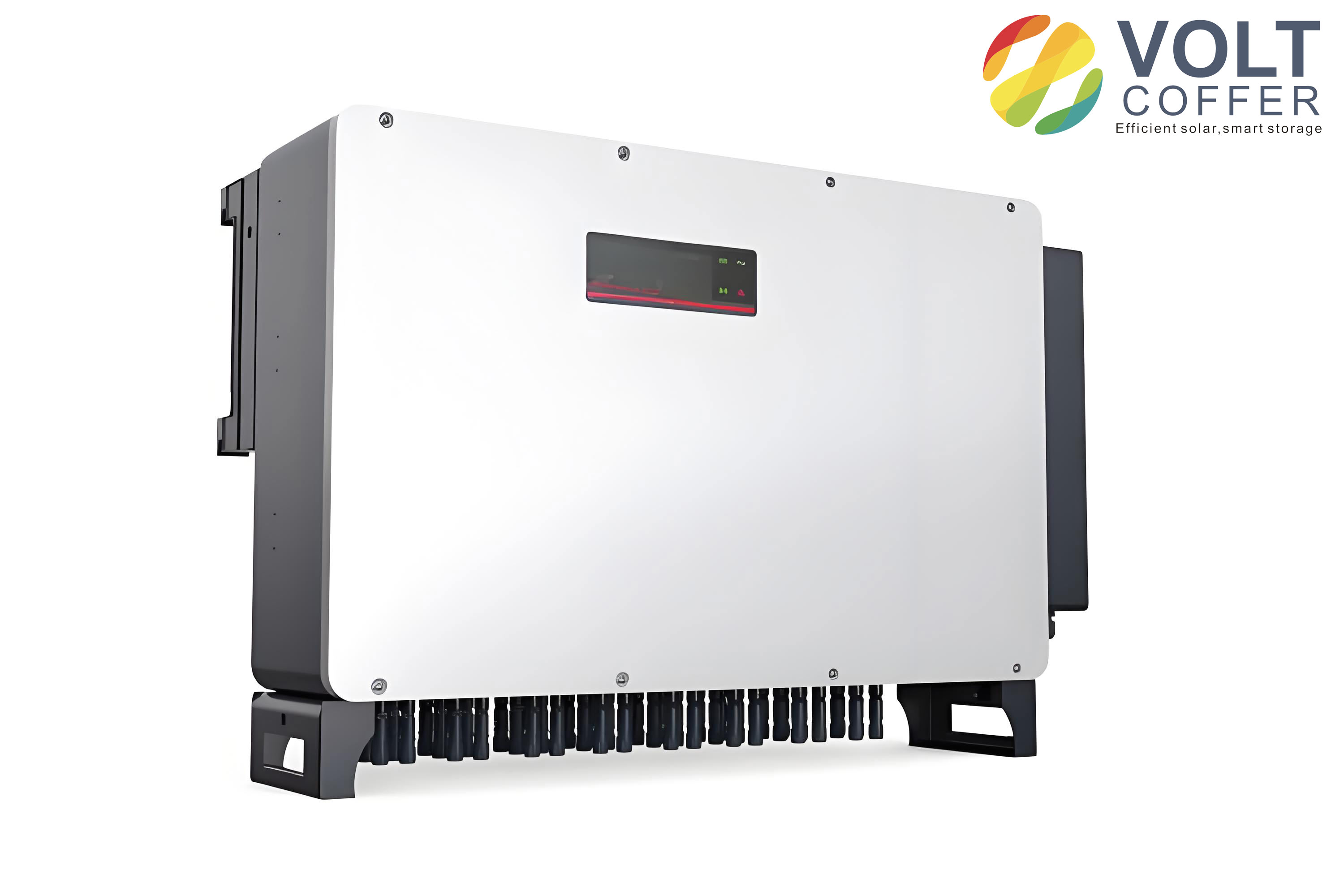
The experimental results confirmed the simulation. At an output power of 1.476 kW, the power factor was 0.998, and the current total harmonic distortion was below 3 percent. The grid current was sinusoidal and in phase with the grid voltage. The waveform quality was high, and the dynamic response was fast. When the grid frequency was changed slightly, the current remained stable and the total harmonic distortion increased only slightly. When the grid voltage was disturbed, the current recovered quickly. These results demonstrate that the improved grid-connected control method is feasible and practical for solar inverters.
| Experimental condition | Measured value |
|---|---|
| Output power | 1.476 kW |
| Grid voltage | 220 V rms |
| Grid frequency | 50 Hz |
| Power factor | 0.998 |
| Current total harmonic distortion | Less than 3 percent |
| Current waveform | Sinusoidal and synchronized |
| Dynamic response | Fast recovery after disturbance |
The improved method has several advantages for solar inverters. First, it eliminates the steady-state amplitude and phase error of the current loop. Second, it reduces the influence of grid-frequency deviation. Third, it lowers the current total harmonic distortion. Fourth, it improves the power factor. Fifth, it maintains fast dynamic response. Sixth, it is compatible with digital signal processors and can be extended with harmonic resonators. These advantages make the quasi-proportional-resonant inner loop a strong candidate for modern single-phase solar inverters.
I also compared the computational burden of the proposed method with the conventional method. The proportional-integral controller requires one integrator and a few multiplications. The quasi-proportional-resonant controller requires a second-order filter section. The multi-resonant version requires one second-order section per harmonic. For a typical digital signal processor used in solar inverters, this is not a significant burden if the number of resonators is limited. In my implementation, I used resonators at the fundamental, third, fifth, and seventh frequencies. This provided a good balance between performance and computational cost. Higher-order resonators can be added if the grid distortion is severe, but they increase the computational load and require careful tuning.
The design procedure I followed can be summarized as follows. First, select the direct-current link voltage, grid voltage, rated power, and switching frequency. Second, design the filter inductance and direct-current link capacitance. Third, design the outer proportional-integral voltage loop with a low bandwidth. Fourth, design the inner quasi-proportional-resonant current loop. Fifth, choose \(K_p\) for phase margin and crossover frequency. Sixth, choose \(K_R\) for high gain at the fundamental frequency. Seventh, choose \(\omega_c\) for frequency tolerance. Eighth, add harmonic resonators if needed. Ninth, discretize the controller and implement it in the digital signal processor. Tenth, verify the design by simulation and experiment. This procedure is general and can be applied to other single-phase solar inverters.
| Design step | Main objective | Key parameter |
|---|---|---|
| Direct-current link | Limit voltage ripple | \(C_{dc}\) |
| Filter | Limit current ripple | \(L_f\) |
| Outer voltage loop | Regulate direct-current voltage | \(K_{pv}, K_{iv}\) |
| Inner current loop | Track sinusoidal current | \(K_p, K_R, \omega_c\) |
| Harmonic resonators | Reduce current distortion | \(K_{R,h}\) |
| Digital implementation | Real-time execution | \(T_s\) |
The phase-locked loop is also important for solar inverters. It provides the grid voltage phase angle \(\theta_g\), which is used to generate the current reference. If the phase-locked loop is inaccurate, the current may not be synchronized with the grid voltage. In my model, I used a synchronous-reference-frame phase-locked loop for the single-phase system. The phase-locked loop output was used to calculate
$$ i_g^*(t)=I_m^*\sin(\theta_g) $$
for unity power factor. When the grid frequency changed, the phase-locked loop tracked the new frequency, and the quasi-proportional-resonant resonant frequency could be updated accordingly. This further improves the robustness of the solar inverter under weak-grid conditions.
I also considered the effect of the direct-current link voltage ripple. In single-phase solar inverters, the instantaneous power oscillates at twice the grid frequency. This causes a voltage ripple on the direct-current link. The outer voltage loop must be slow enough to avoid injecting this ripple into the current reference. If the outer loop bandwidth is too high, the current reference will contain a second-harmonic component, which distorts the grid current. I therefore set the outer loop bandwidth well below the second harmonic of the grid frequency. The quasi-proportional-resonant inner loop then tracks the fundamental current reference accurately. This separation of bandwidths is essential for high-quality operation of solar inverters.
The current controller output is used by the pulse-width modulator. The modulator generates the gate signals for the full-bridge inverter. The inverter output voltage contains switching harmonics, which are attenuated by the filter. The quasi-proportional-resonant controller does not eliminate switching harmonics directly, but it reduces low-order harmonics and ensures accurate fundamental tracking. The filter design must still attenuate the switching frequency components. In my design, the filter inductance was selected to keep the switching ripple within an acceptable range. The switching frequency was 20 kHz, which is above the audible range and allows a relatively small filter. This is common in modern solar inverters.
The total harmonic distortion of the grid current is a key figure of merit. In my simulation, the quasi-proportional-resonant controller achieved a total harmonic distortion of about 2.58 percent. In the experiment, the total harmonic distortion was below 3 percent at 1.476 kW. These values satisfy typical grid-code requirements for solar inverters. The power factor was 0.998, which is close to unity. The current waveform was smooth and synchronized with the grid voltage. The dynamic response was fast, with recovery times on the order of one millisecond after a disturbance. These results confirm the effectiveness of the improved control method.
The improved method can also be applied to three-phase solar inverters, although the coordinate transformations differ. In a three-phase system, the quasi-proportional-resonant controller can be implemented in the stationary reference frame for each phase or in the synchronous reference frame with proportional-integral controllers plus harmonic compensators. The principle is the same: use resonant terms to achieve zero steady-state error at the fundamental and selected harmonic frequencies. For single-phase solar inverters, the stationary-frame implementation is natural because there is only one alternating-current quantity. The quasi-proportional-resonant controller is therefore particularly well suited to single-phase solar inverters.
I also note that the quasi-proportional-resonant controller is not a universal solution. It requires careful tuning. If \(K_R\) is too large, the resonant peak may cause excessive oscillation or reduce the phase margin. If \(\omega_c\) is too small, the controller may not tolerate grid-frequency deviation. If \(\omega_c\) is too large, the resonant term becomes broad and loses selectivity. If harmonic resonators are added without proper damping, they can interact with each other and with the fundamental resonator. Therefore, I tuned the parameters iteratively using frequency-response analysis and time-domain simulation. This is the practical approach for solar inverters, where safety, stability, and power quality are all important.
The proposed controller can be expressed in a compact form as
$$ u(s)=\left[K_p+\sum_{h\in\{1,3,5,7\}}\frac{2K_{R,h}\omega_c s}{s^2+2\omega_c s+(h\omega_0)^2}\right]\left(i_g^*(s)-i_g(s)\right) $$
where \(u(s)\) is the controller output, \(i_g^*(s)\) is the reference grid current, and \(i_g(s)\) is the measured grid current. In a digital implementation, the measured current is sampled at \(T_s\), and the controller output is updated once per sampling period. The pulse-width modulator then generates the switching signals. This structure is simple, modular, and suitable for solar inverters.
The outer voltage loop can be written as
$$ I_m^*(s)=\left(K_{pv}+\frac{K_{iv}}{s}\right)\left(V_{dc}^*(s)-V_{dc}(s)\right) $$
This generates the current amplitude command. The phase-locked loop generates the phase command. The inner current loop then forces the actual current to follow the reference. The improved inner loop is the key contribution. It provides zero steady-state error, low harmonic distortion, and robustness to grid-frequency variation. These are exactly the requirements for high-performance solar inverters.
In conclusion, I have developed an improved grid-connected control method for single-phase solar inverters. The method uses a proportional-integral outer voltage loop and a quasi-proportional-resonant inner current loop. The quasi-proportional-resonant controller provides very high gain at the fundamental frequency and can be extended with harmonic resonators. It eliminates the steady-state current error that occurs with a proportional-integral inner loop and reduces the effect of grid-frequency deviation. I established a simulation model and verified the design with experiments. The results show that the improved control method achieves a sinusoidal grid current, low total harmonic distortion, high power factor, fast dynamic response, and strong robustness. The total harmonic distortion was about 2.58 percent in simulation and below 3 percent in experiment. The power factor was 0.998 at 1.476 kW. These results confirm that the improved method is feasible and practical for solar inverters. The method can be implemented on a digital signal processor and can be extended to harmonic compensation. It provides a reliable solution for high-quality grid connection of single-phase solar inverters.