
I designed, analyzed, and tested a non-isolated two-stage series solar inverter for small and medium photovoltaic power plants. This solar inverter converts the DC electricity produced by PV modules into AC electricity that is synchronized with the public grid. My main objective was to improve output power quality, conversion efficiency, reliability, and safety while reducing cost and volume. I selected an interleaved Boost converter as the front-end stage and an H6 inverter bridge as the rear-end stage. The front-end stage performs voltage boosting and maximum power point tracking, while the rear-end stage performs DC-AC inversion, grid current control, and common-mode leakage current suppression. I used a variable-step incremental conductance method for maximum power point tracking and a quasi-proportional resonant controller for grid current regulation. I validated the complete solar inverter design through MATLAB/Simulink simulations and a laboratory prototype.
The solar inverter is the central interface between a PV array and the utility grid. Its behavior determines whether the PV system delivers clean, stable, and efficient power. In a non-isolated solar inverter, the absence of a transformer reduces size, weight, and cost, but it also creates a galvanic connection between the PV array and the grid. This connection makes common-mode leakage current a critical design issue. Therefore, I focused on both conversion topology and modulation strategy to suppress leakage current while maintaining high differential-mode performance. The term solar inverter appears throughout this design because every major decision is related to the grid-tied operation of the solar inverter.
Background and Design Motivation
Solar energy is clean, abundant, safe, and geographically flexible. Unlike fossil fuels, it does not produce direct emissions during operation, and it can serve remote areas that are not covered by the main grid. However, the cost of PV generation remains sensitive to component efficiency and system reliability. For a solar inverter, efficiency and reliability are not abstract goals. They directly affect the amount of energy harvested, the payback period, and the stability of the public grid. I therefore treated the solar inverter as a system-level problem rather than a simple power converter.
In recent years, string or series solar inverter architectures have become dominant in small and medium PV installations. A series solar inverter usually connects a limited number of PV panels to one power conversion unit. This arrangement provides distributed maximum power point tracking, easier maintenance, and better tolerance to partial shading than a centralized solar inverter. When one series solar inverter fails, the remaining units can continue to operate. In contrast, a centralized solar inverter may cause a large fraction of the plant to stop. I selected a series solar inverter architecture because it matches the needs of small and medium systems and because it allows me to apply advanced MPPT and current control methods per string.
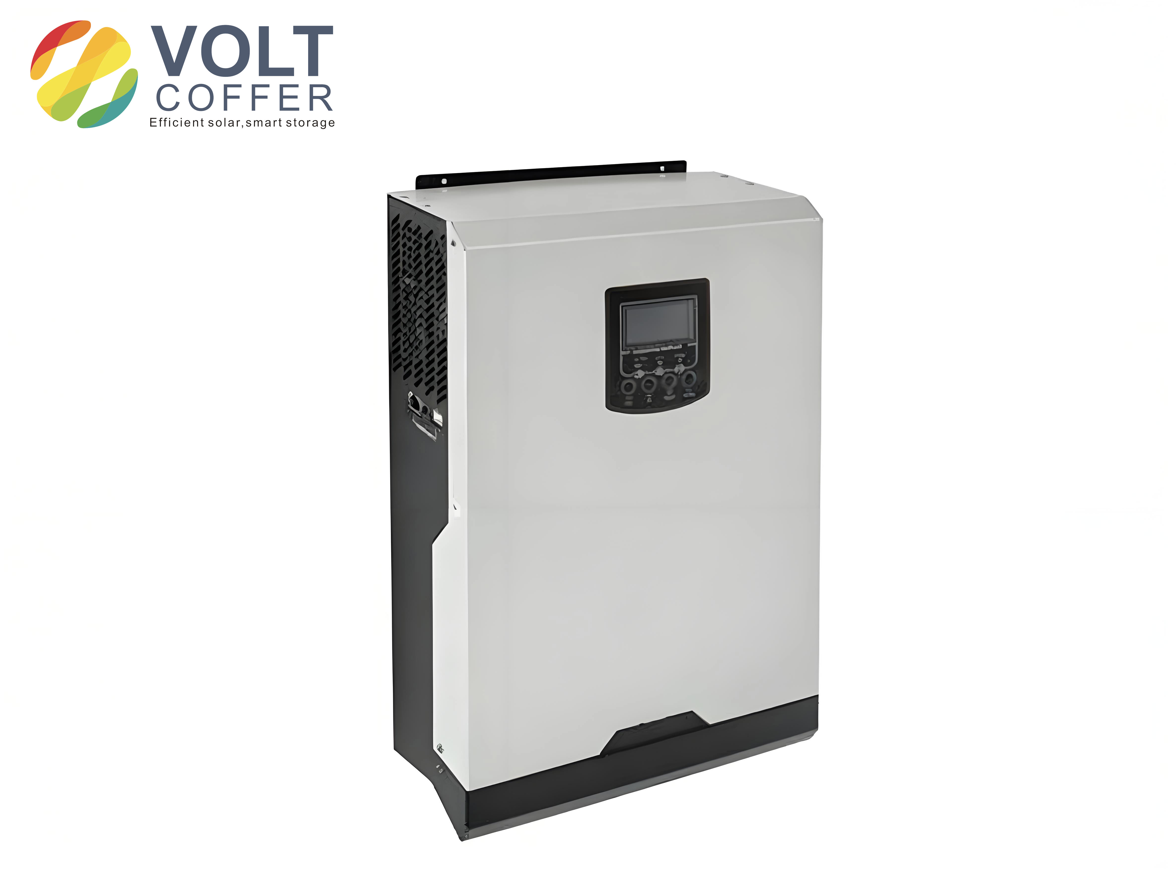
A solar inverter can be classified in several ways. The classification affects the topology, control complexity, isolation requirement, and grid interface. I summarized the main categories in the following table and indicated my design choice.
| Classification Criterion | Type | Main Features | My Choice |
|---|---|---|---|
| Power conversion stages | Single-stage solar inverter | Boost, MPPT, and inversion occur in one stage; simple structure but complex control. | Not selected. |
| Power conversion stages | Two-stage solar inverter | Front-end DC-DC performs boost and MPPT; rear-end DC-AC performs inversion and grid current control. | Selected. |
| Isolation | Isolated solar inverter | Line-frequency or high-frequency transformer provides galvanic isolation; larger and more expensive. | Not selected. |
| Isolation | Non-isolated solar inverter | No transformer; smaller, lighter, and potentially more efficient; leakage current must be controlled. | Selected. |
| Grid connection | Grid-tied solar inverter | Output current is synchronized with grid voltage; anti-islanding and grid support may be required. | Selected. |
| Grid connection | Off-grid solar inverter | Supplies local loads or battery storage; voltage control is often used. | Not selected. |
| System architecture | Central solar inverter | Large central converter; lower cost per watt but weak tolerance to mismatch and failure. | Not selected. |
| System architecture | Series or string solar inverter | Distributed MPPT, modular maintenance, better shading tolerance, and high energy yield. | Selected. |
I designed the solar inverter to meet a set of practical specifications. The maximum output power is 1 kW, the PV input voltage ranges from 100 V to 300 V, the rated grid voltage is 220 V, the maximum output current is 4.5 A, the rated grid frequency is 50 Hz with a tolerance of ±1%, and the current total harmonic distortion must be no greater than 5%. These specifications guided the component ratings, control bandwidth, filter design, and protection thresholds.
Front-End Interleaved Boost Converter
I selected an interleaved Boost converter as the front-end stage of the solar inverter. A conventional Boost converter can boost the PV voltage and implement MPPT, but its input current ripple is relatively large. Large input current ripple increases conduction loss, induces electromagnetic interference, and may reduce MPPT accuracy. An interleaved Boost converter uses two parallel Boost cells whose gate signals have the same switching period and a phase difference of \(180^\circ\). The total input current is the sum of the two inductor currents. Because the two currents rise and fall in an alternating manner, their ripples partially cancel. This property improves the input current quality and reduces the required input capacitance. For a solar inverter, this means faster dynamic response and better reliability.
The topology contains two equal inductors \(L_1\) and \(L_2\), two power switches \(S_1\) and \(S_2\), two diodes \(D_1\) and \(D_2\), and one output capacitor. The converter operates in continuous conduction mode. I analyzed two duty-ratio ranges: \(0 \lt D \le 0.5\) and \(0.5 \lt D \lt 1\).
For \(0 \lt D \le 0.5\), the equivalent duty ratio of the summed current is
$$D_1 = 2D$$
The total input current ripple is
$$\Delta i_L = \frac{V_o D(1-2D)T}{L}$$
For \(0.5 \lt D \lt 1\), the equivalent duty ratio is
$$D_2 = 2D – 1$$
The total input current ripple is
$$\Delta i_L = \frac{V_o (1-D)(2D-1)T}{L}$$
For comparison, a conventional Boost converter has an input current ripple of
$$\Delta I_1 = \frac{V_o D(1-D)T}{L}$$
I summarized the ripple behavior of the two converters in the following table.
| Duty Ratio Range | Conventional Boost Ripple | Interleaved Boost Ripple | Observation |
|---|---|---|---|
| \(0 \lt D \le 0.5\) | \(\frac{V_o D(1-D)T}{L}\) | \(\frac{V_o D(1-2D)T}{L}\) | The interleaved ripple is smaller for the same \(D\). |
| \(0.5 \lt D \lt 1\) | \(\frac{V_o D(1-D)T}{L}\) | \(\frac{V_o (1-D)(2D-1)T}{L}\) | The interleaved ripple remains smaller and reaches zero at \(D=0.5\). |
| \(D=0.5\) | \(\frac{V_o(0.5)(0.5)T}{L}\) | \(0\) | The two inductor ripples cancel completely. |
I also analyzed the switching modes. For \(0 \lt D \le 0.5\), there are three modes. In the first mode, \(S_1\) and \(D_2\) conduct, \(i_{L1}\) rises, and \(i_{L2}\) falls. In the second mode, \(S_2\) and \(D_1\) conduct, \(i_{L2}\) rises, and \(i_{L1}\) falls. In the third mode, both switches are off and both diodes conduct, so both inductor currents fall. For \(0.5 \lt D \lt 1\), there are also three modes. In one mode, one switch and one diode conduct. In another mode, the other switch and the other diode conduct. In the third mode, both switches conduct and both diodes are off, so both inductor currents rise. These modes confirm that the interleaved structure distributes current stress and reduces the total ripple.
| Duty Ratio | Mode | Conducting Devices | Inductor Current Behavior | Input Current Trend |
|---|---|---|---|---|
| \(0 \lt D \le 0.5\) | Mode 1 | \(S_1\), \(D_2\) | \(i_{L1}\) rises, \(i_{L2}\) falls | Rises |
| \(0 \lt D \le 0.5\) | Mode 2 | \(S_2\), \(D_1\) | \(i_{L1}\) falls, \(i_{L2}\) rises | Rises |
| \(0 \lt D \le 0.5\) | Mode 3 | \(D_1\), \(D_2\) | Both currents fall | Falls |
| \(0.5 \lt D \lt 1\) | Mode 4 | \(S_1\), \(D_2\) | \(i_{L1}\) rises, \(i_{L2}\) falls | Falls |
| \(0.5 \lt D \lt 1\) | Mode 5 | \(S_2\), \(D_1\) | \(i_{L1}\) falls, \(i_{L2}\) rises | Falls |
| \(0.5 \lt D \lt 1\) | Mode 6 | \(S_1\), \(S_2\) | Both currents rise | Rises |
I built simulation models for both the conventional Boost converter and the interleaved Boost converter. I set \(L_1=L_2=1\) mH, a switching frequency of 20 kHz, and a load of 50 \(\Omega\). When the input voltage was 250 V and the duty ratio was 0.375, the interleaved Boost converter produced a smaller input current ripple. When the input voltage was 200 V and the duty ratio was 0.5, the input current ripple of the interleaved converter was almost eliminated. The output voltage fluctuation was also narrower. These simulation results confirmed the theoretical analysis and showed that the interleaved Boost converter is a strong front-end choice for a solar inverter.
Solar Cell Model and Maximum Power Point Tracking
To design MPPT for the solar inverter, I first modeled the solar cell. A solar cell behaves as a nonlinear current source whose output depends on irradiance and temperature. The equivalent circuit includes a photocurrent source, a diode, a series resistance, and a shunt resistance. The output current-voltage relationship can be written as
$$I = I_{ph} – I_o \left[ \exp\left( \frac{q(U+IR_s)}{AKT} \right) – 1 \right] – \frac{U+IR_s}{R_{sh}}$$
Here, \(I_{ph}\) is the photocurrent, \(I_o\) is the diode reverse saturation current, \(R_s\) is the series resistance, \(R_{sh}\) is the shunt resistance, \(A\) is the diode ideality factor, \(K\) is Boltzmann’s constant, \(T\) is the absolute temperature, and \(q\) is the elementary charge. For practical modeling, I used the following simplified form based on the short-circuit current \(I_{sc}\) and open-circuit voltage \(U_{oc}\):
$$I = I_{sc} \left[ 1 – C_1 \left( \exp\left( \frac{U}{C_2 U_{oc}} \right) – 1 \right) \right]$$
$$C_1 = \left( 1 – \frac{I_m}{I_{sc}} \right) \exp\left( -\frac{U_m}{C_2 U_{oc}} \right)$$
$$C_2 = \left( \frac{U_m}{U_{oc}} – 1 \right) \left[ \ln\left( 1 – \frac{I_m}{I_{sc}} \right) \right]^{-1}$$
I also included temperature and irradiance effects:
$$\Delta V = \beta(T – T_{ref}) – R_s \Delta I$$
$$\Delta I = \alpha \frac{S}{S_{ref}}(T – T_{ref}) + \left( \frac{S}{S_{ref}} – 1 \right) I_{sc}$$
In these equations, \(S\) is the irradiance, \(S_{ref}\) is the reference irradiance, \(T\) is the cell temperature, \(T_{ref}\) is the reference temperature, \(\alpha\) is the current temperature coefficient, and \(\beta\) is the voltage temperature coefficient. The P-U and I-U curves show a single maximum power point under uniform conditions. As irradiance increases, the maximum power increases. As temperature increases, the maximum power usually decreases. Therefore, the solar inverter must track the maximum power point continuously.
The principle of MPPT can be understood from the impedance matching viewpoint. When the PV array output resistance equals the equivalent resistance of the rear-end circuit, the PV array delivers maximum power. For a Boost-type front-end, the relationship between the PV output resistance and the duty ratio is
$$R_{pv} = (1-D)^2 R$$
Thus, by adjusting the duty ratio \(D\), I can shift the operating point of the PV array. If the operating point is on the left side of the maximum power point, I reduce \(D\) to increase \(R_{pv}\). If the operating point is on the right side, I increase \(D\) to decrease \(R_{pv}\). This is the basis of MPPT in the solar inverter.
I reviewed several MPPT methods. The following table compares their principles and practical trade-offs.
| MPPT Method | Basic Principle | Advantages | Drawbacks |
|---|---|---|---|
| PV array combination method | Change series-parallel configuration of panels. | Simple concept. | Poor real-time tracking and limited flexibility. |
| Constant voltage method | Force PV voltage to a fixed fraction of open-circuit voltage. | Simple and fast. | Not a true tracking method; weak under temperature variation. |
| Open-circuit voltage or short-circuit current ratio | Use approximate linear relationship at MPP. | Simple implementation. | Requires periodic interruption; accuracy is limited. |
| Perturb and observe | Perturb voltage and observe power change. | Easy to implement. | Oscillation around MPP; possible misjudgment under fast irradiance change. |
| Incremental conductance | Use \(\frac{dP}{dU}=0\) at MPP. | Good steady-state accuracy. | Fixed step size creates a speed-accuracy conflict. |
| Variable-step incremental conductance | Adjust step size according to \(\frac{dP}{dU}\). | Fast dynamic response and good steady-state precision. | Requires careful scaling and stable implementation. |
| Neural network or sliding mode | Use artificial intelligence or nonlinear control. | Potential for strong performance. | Complex, data-dependent, and costly. |
I selected the variable-step incremental conductance method for the solar inverter. The output power is
$$P = UI$$
Differentiating with respect to voltage gives
$$\frac{dP}{dU} = I + U \frac{dI}{dU}$$
At the maximum power point,
$$\frac{dP}{dU} = 0$$
Therefore,
$$\frac{I}{U} = -\frac{dI}{dU}$$
If \(\frac{I}{U} \gt -\frac{dI}{dU}\), the operating point is on the left side of the MPP. If \(\frac{I}{U} \lt -\frac{dI}{dU}\), the operating point is on the right side. I used a variable step to avoid the trade-off between speed and accuracy. The duty-ratio update law is
$$D(t) = D(t-1) \pm N \left| \frac{P(t)-P(t-1)}{U(t)-U(t-1)} \right|$$
Here, \(N\) is a scaling factor. When the operating point is far from the MPP, the step is large, so the tracking speed is high. When the operating point is close to the MPP, the step becomes small, so steady-state oscillation is reduced. I also used an initial fixed step \(\Delta D_{max}\) to shorten the startup time. The scaling factor must satisfy
$$N \left| \frac{dP}{dU} \right|_{max} \lt \Delta D_{max}$$
I simulated the conventional incremental conductance method and the variable-step incremental conductance method. The variable-step method reached the maximum power point at about 0.03 s and then remained stable. The conventional method required a longer time and showed more power fluctuation. I also changed the irradiance from 1000 W/m\(^2\) to 1200 W/m\(^2\) and then to 800 W/m\(^2\) while keeping the temperature constant. The variable-step method tracked the new maximum power point quickly and accurately. The output power, voltage, and current were proportional to irradiance, which confirmed the expected behavior of the solar inverter under changing conditions.
| Test Condition | Observed MPPT Response | Implication for the Solar Inverter |
|---|---|---|
| Startup at 1000 W/m\(^2\) | Reached MPP near 0.03 s. | Fast initial energy capture. |
| Step-up irradiance to 1200 W/m\(^2\) | Power increased and MPP was tracked quickly. | Good dynamic response under increasing solar input. |
| Step-down irradiance to 800 W/m\(^2\) | Power decreased and MPP was tracked without sustained oscillation. | Stable operation under shading or cloud passage. |
| Steady irradiance | Power remained close to the MPP with small ripple. | High steady-state efficiency. |
Rear-End H6 Inverter Bridge
The rear-end stage of the solar inverter converts the DC bus voltage into grid-compatible AC current. In a non-isolated solar inverter, the PV array and the grid are not galvanically isolated. A parasitic capacitance exists between the PV array and ground. This capacitance provides a path for common-mode leakage current. Excessive leakage current can cause electromagnetic interference, increase current distortion, reduce efficiency, and create safety hazards. Therefore, I selected the H6 inverter bridge because it can suppress common-mode leakage current while maintaining good differential-mode characteristics.
For a full-bridge inverter, the differential-mode voltage and common-mode voltage are defined as
$$U_{DM} = U_{AN} – U_{BN}$$
$$U_{CM} = \frac{U_{AN} + U_{BN}}{2}$$
The common-mode leakage current is approximately
$$i_{CM} = C_{pv} \frac{dU_{CM}}{dt}$$
Here, \(C_{pv}\) is the parasitic capacitance between the PV array and ground. If \(U_{CM}\) is constant, the leakage current is theoretically zero. This is the key requirement for a non-isolated solar inverter. I compared several transformerless inverter topologies in the following table.
| Topology | Common-Mode Voltage Behavior | Differential-Mode Output | Leakage Current | Efficiency Trend |
|---|---|---|---|---|
| H4 with unipolar SPWM | \(U_{CM}\) jumps at high frequency. | Three-level output. | Large. | High switch efficiency but poor leakage performance. |
| H4 with bipolar SPWM | \(U_{CM}\) is constant. | Two-level output. | Small. | Higher switching loss and larger ripple. |
| H5 | \(U_{CM}\) is nearly constant. | Three-level output. | Small. | High efficiency but uneven loss distribution. |
| Heric | \(U_{CM}\) is nearly constant. | Three-level output. | Small. | Good efficiency with extra AC-side switches. |
| Six-switch bridge | \(U_{CM}\) is constant. | Three-level output. | Small. | Good performance but more components. |
| H6 bridge | \(U_{CM}\) remains \(U_{dc}/2\). | Three-level output. | Very small. | High efficiency and reactive power capability. |
The H6 inverter bridge uses six switches. It can operate in four time intervals and six switching modes. During the positive half-cycle, one switch remains on, and two switches are modulated. During the negative half-cycle, another switch remains on, and two other switches are modulated. The H6 bridge maintains the common-mode voltage at \(U_{dc}/2\) even when reactive power is injected into the grid. This is important because modern grid standards often require the solar inverter to provide reactive power support.
I analyzed the six modes of the H6 bridge. The key voltages are summarized below.
| Mode | Conducting Devices | \(U_{AN}\) | \(U_{BN}\) | \(U_{CM}\) | \(U_{DM}\) |
|---|---|---|---|---|---|
| Mode 1 | \(S_1\), \(S_4\), \(S_6\) | \(U_{dc}\) | 0 | \(U_{dc}/2\) | \(U_{dc}\) |
| Mode 2 | \(S_5\), \(S_6\) | \(U_{dc}/2\) | \(U_{dc}/2\) | \(U_{dc}/2\) | 0 |
| Mode 3 | \(S_2\), \(S_3\), \(S_5\) | 0 | \(U_{dc}\) | \(U_{dc}/2\) | \(-U_{dc}\) |
| Mode 4 | \(S_2\), \(S_3\), \(S_5\) | 0 | \(U_{dc}\) | \(U_{dc}/2\) | \(-U_{dc}\) |
| Mode 5 | \(S_5\), \(S_6\) | \(U_{dc}/2\) | \(U_{dc}/2\) | \(U_{dc}/2\) | 0 |
| Mode 6 | \(S_1\), \(S_4\), \(S_6\) | \(U_{dc}\) | 0 | \(U_{dc}/2\) | \(U_{dc}\) |
I simulated the H6 inverter bridge with a DC bus voltage of 400 V, an output voltage of 220 V at 50 Hz, filter inductors of 3 mH, a filter capacitor of 2.2 \(\mu\)F, and a PV parasitic capacitance of 50 nF. The differential-mode voltage showed a three-level waveform, and the common-mode voltage remained near 200 V with little oscillation. I also simulated an H4 bridge with unipolar SPWM for comparison. The H4 leakage current reached about 1.5 A, while the H6 leakage current was nearly 0 A. This confirmed that the H6 bridge is effective for suppressing common-mode leakage current in a non-isolated solar inverter.
Grid Current Control and Quasi-Proportional Resonant Control
The grid current control loop determines the quality of the AC current injected by the solar inverter. Because the grid voltage clamps the inverter output voltage, the solar inverter is usually controlled as a current source. The controller must force the output current to follow a sinusoidal reference that is synchronized with the grid voltage. I modeled the inverter stage as a high-gain small inertia element:
$$G_{inv}(s) = \frac{K}{Ts+1} \approx K$$
The filter inductor and equivalent resistance form the plant:
$$G_f(s) = \frac{1}{Ls+R}$$
The open-loop plant is therefore
$$G(s) = G_{inv}(s)G_f(s) = \frac{K}{Ls+R}$$
I compared several current control methods. The following table summarizes their properties.
| Control Method | Principle | Advantages | Limitations |
|---|---|---|---|
| Deadbeat control | Predict the next current from the model and force zero error. | Fast dynamic response and high accuracy. | Very sensitive to model errors and parameter mismatch. |
| Hysteresis control | Switch when current error exceeds a band. | Fast response and simple concept. | Variable switching frequency; difficult filter design. |
| Repetitive control | Correct periodic errors from previous cycles. | Excellent suppression of periodic distortion. | Slow dynamic response; often combined with PI control. |
| PI control | Proportional and integral action on current error. | Simple and widely used. | Steady-state amplitude and phase error at the fundamental frequency. |
| PR control | Add a resonant term at the grid frequency. | Theoretically zero steady-state error at the fundamental frequency. | Narrow bandwidth and sensitive to grid frequency deviation. |
| QPR control | Add a damped resonant term at the grid frequency. | High gain, wider bandwidth, and better frequency tolerance. | Requires careful parameter selection. |
The PI controller transfer function is
$$G_{PI}(s) = K_P + \frac{K_I}{s}$$
Although PI control is simple, it cannot completely eliminate steady-state error when tracking a sinusoidal reference. The PR controller introduces a resonant term:
$$G_{PR}(s) = K_P + \frac{2K_R s}{s^2+\omega_0^2}$$
At the fundamental frequency \(\omega_0\), the PR controller has infinite gain, so it can achieve zero steady-state error in theory. However, its bandwidth is narrow. If the grid frequency deviates from 50 Hz, the gain drops quickly, and the control performance degrades. To solve this problem, I selected the quasi-proportional resonant controller:
$$G_{QPR}(s) = K_P + \frac{2K_R \omega_c s}{s^2+2\omega_c s+\omega_0^2}$$
Here, \(K_P\) is the proportional gain, \(K_R\) is the resonant gain, \(\omega_0\) is the fundamental angular frequency, and \(\omega_c\) is the cutoff frequency. The cutoff frequency determines the bandwidth. I allowed the grid frequency to vary within 50 ± 0.5 Hz, so the bandwidth was 1 Hz. Therefore, I chose \(\omega_c = \pi \times 1 = 3.14\) rad/s. I selected \(K_P = 2.5\), \(K_R = 50\), and \(\omega_0 = 314\) rad/s.
| Parameter | Value | Role in the Solar Inverter Controller |
|---|---|---|
| \(K_P\) | 2.5 | Improves transient response and overall stiffness. |
| \(K_R\) | 50 | Provides high gain at the grid frequency. |
| \(\omega_0\) | 314 rad/s | Fundamental frequency for a 50 Hz grid. |
| \(\omega_c\) | 3.14 rad/s | Widens the resonant peak to tolerate frequency drift. |
I simulated the solar inverter with PI, PR, and QPR controllers. Under normal grid frequency, the PI controller produced a current THD of 4.28%, while the QPR controller produced a current THD of 2.16%. When the grid frequency shifted to 49.5 Hz, the PR controller produced a current THD of 7.71%, while the QPR controller produced a current THD of 4.07%. These results showed that the QPR controller provides better steady-state accuracy and better tolerance to grid frequency variation. Therefore, I used QPR control in the final solar inverter design.
| Controller | Grid Condition | Current THD | Assessment |
|---|---|---|---|
| PI | 50 Hz | 4.28% | Meets the limit but has larger steady-state error. |
| QPR | 50 Hz | 2.16% | Better current quality and lower distortion. |
| PR | 49.5 Hz | 7.71% | Exceeds desirable limits under frequency drift. |
| QPR | 49.5 Hz | 4.07% | Maintains acceptable performance under frequency drift. |
Hardware and Software Design
I built the solar inverter around a TMS320F28335 digital signal processor. The processor executes the MPPT algorithm, the QPR current control law, the SPWM generation, and the digital phase-locked loop. The main circuit includes the interleaved Boost front-end, the H6 inverter bridge, the DC bus capacitor, and the output filter. The peripheral circuits include PV voltage and current sensing, DC bus voltage sensing, grid voltage and output current sensing, zero-crossing detection, gate drive circuits, overcurrent protection, and auxiliary power supplies.
The main design parameters of the solar inverter are listed below.
| Parameter | Value |
|---|---|
| Maximum output power | 1 kW |
| PV input voltage | 100 V to 300 V |
| Rated grid voltage | 220 V |
| Maximum output current | 4.5 A |
| Rated grid frequency | 50 Hz ± 1% |
| Current THD requirement | ≤ 5% |
| DC bus voltage | 400 V |
| Switching frequency | 20 kHz |
For the front-end interleaved Boost stage, I selected components based on voltage and current stress. The switches and diodes must block the DC bus voltage, which is 400 V. After allowing margin, I selected 600 V devices. The maximum input current is about 10 A, so each Boost phase carries about 5 A. With a 20% ripple margin, each phase carries about 6 A. After allowing margin, I selected devices with current ratings between 9 A and 15 A. I used two SGH40N60UFD IGBTs and two RURP1560 fast recovery diodes. The inductors were 1 mH each, wound on iron-silicon-aluminum toroidal cores with 0.7 mm wire.
| Front-End Component | Selected Device or Value | Voltage Rating | Current Rating |
|---|---|---|---|
| Boost switches | Two SGH40N60UFD IGBTs | 600 V | 20 A |
| Boost diodes | Two RURP1560 fast recovery diodes | 600 V | 15 A |
| Boost inductors | 1 mH each | Not applicable | Rated for phase current |
For the rear-end H6 inverter bridge, the switches must block the 400 V DC bus. After margin, I selected 600 V devices. The maximum current through the switches is approximately
$$I_{max} = \frac{\sqrt{2}P}{U_{g,min}}$$
With \(P=1000\) W and \(U_{g,min}=200\) V, the maximum current is about 7.07 A. After a 20% ripple margin, the current is about 9 A. After further margin, I selected devices rated between 15 A and 30 A. I used six STGW20NC60VD IGBTs, which have a 600 V blocking voltage and a 30 A collector current. For the DC bus, I calculated the required capacitance as
$$C_{dc} = \frac{P}{\omega_0 U_{dc} U_r}$$
I used \(P=1000\) W, \(\omega_0=314\) rad/s, \(U_{dc}=400\) V, and a ripple voltage \(U_r\) equal to 5% of the DC bus voltage, or 20 V. The calculated capacitance was about 398 \(\mu\)F. After margin, I selected a 1000 \(\mu\)F electrolytic capacitor.
| Rear-End Component | Selected Device or Value | Voltage Rating | Current Rating |
|---|---|---|---|
| H6 switches | Six STGW20NC60VD IGBTs | 600 V | 30 A |
| DC bus capacitor | 1000 \(\mu\)F electrolytic capacitor | 400 V or higher | Ripple current rated |
For the output filter, I used two inductors and one capacitor. The sum of the two filter inductors is determined by the maximum output current ripple:
$$L_{f1}+L_{f2} = \frac{U_{dc} \Delta_{factor}}{f \Delta i}$$
The ripple factor is
$$\Delta_{factor} = \sin^2(\omega_0 t) – M^2 \sin^2(\omega_0 t)$$
I selected a modulation index \(M=0.8\), a maximum current ripple \(\Delta i=1\) A, and a switching frequency \(f=20\) kHz. The calculated sum of the inductances was about 5 mH. I selected \(L_{f1}=L_{f2}=3\) mH. The filter capacitor is chosen from the cutoff frequency:
$$C_f = \frac{1}{4\pi^2 f_s^2 L_f}$$
I selected a cutoff frequency \(f_s=2\) kHz. The calculated capacitance was about 2 \(\mu\)F, and I used 2.2 \(\mu\)F in the prototype.
| Filter Parameter | Symbol | Value |
|---|---|---|
| Filter inductor 1 | \(L_{f1}\) | 3 mH |
| Filter inductor 2 | \(L_{f2}\) | 3 mH |
| Filter capacitor | \(C_f\) | 2.2 \(\mu\)F |
| Switching frequency | \(f\) | 20 kHz |
| Cutoff frequency | \(f_s\) | 2 kHz |
I also designed the sensing and protection circuits. The PV voltage sensing circuit uses a resistor divider to scale the PV voltage into the 0 V to 3.3 V range of the DSP analog-to-digital converter. The relationship is
$$u_{pv} = \frac{R_2}{R_1+R_2} U_{pv}$$
A clamping circuit with Schottky diodes protects the analog input. The PV current sensing circuit uses an LA55-P current transducer. Its output current is converted to a voltage by a resistor and then amplified. The relationship is
$$u_{ipv} = \frac{I_{pv}}{1000} R_i \frac{R_7}{R_3}$$
The grid voltage sensing circuit uses a differential sampling network and an offset voltage of 1.5 V. The relationship is
$$u_g = \frac{R_{18}}{R_{13}+R_{14}+R_{15}+R_{16}} U_g + 1.5 \text{ V}$$
The output current sensing circuit uses a similar current transducer and offset network:
$$u_{ig} = \frac{i_g}{1000} R_{21} \frac{R_{25}}{R_{23}} + 1.5 \text{ V}$$
The zero-crossing detection circuit converts the grid voltage signal into a square wave. The DSP captures the rising and falling edges through the eCAP module. This information is used by the digital phase-locked loop to obtain the grid frequency and phase. For the gate drive circuits, I used EXB841 drivers for the front-end IGBTs and 6N137 optocouplers with IR2110 drivers for the rear-end IGBTs. The self-bootstrap capacitor for the IR2110 is chosen as
$$C_{13} \gt \frac{2Q_g}{VCC – V_T – V_{TH}}$$
With \(Q_g=140\) nC, \(VCC=15\) V, \(V_T=10\) V, and \(V_{TH}=1.5\) V, I selected \(C_{13}=0.1\) \(\mu\)F. The overcurrent protection threshold was set to 4.6 A. When the output current exceeds this value, the protection circuit disables the IR2110 outputs and turns off the rear-end switches.
| Peripheral Circuit | Main Device or Method | Purpose |
|---|---|---|
| PV voltage sensing | Resistor divider and clamp | Provide PV voltage to MPPT. |
| PV current sensing | LA55-P current transducer | Provide PV current to MPPT. |
| Grid voltage sensing | Differential amplifier with 1.5 V offset | Measure grid voltage amplitude. |
| Output current sensing | LA55-P current transducer | Measure grid current for QPR control. |
| Zero-crossing detection | LM319 comparator with hysteresis | Provide grid phase information. |
| Front-end gate drive | EXB841 | Drive interleaved Boost IGBTs. |
| Rear-end gate drive | 6N137 and IR2110 | Drive H6 bridge IGBTs. |
| Overcurrent protection | LM319 and TLP521 | Disable gate drives during overcurrent. |
| Auxiliary power | L7820, LM7815, LM7915, LM7805, MCP1700 | Provide +20 V, ±15 V, +5 V, and +3.3 V. |
For the SPWM generation, I used the ePWM module of the DSP. The time-base counter emulates a triangular carrier in up-down mode. The period register is
$$TBPRD = \frac{T_{BCLK}}{T_c}$$
With a 150 MHz system clock and a 20 kHz carrier, the period register was set to 3750. I used symmetric regular sampling. The pulse width is
$$t_{on} = T_c \left[ 0.5 + \frac{M}{2} \sin(\omega_m t_D) \right]$$
For the \(k\)-th sampling point,
$$t_{on,k} = 0.5T_c \left[ 1 + M \sin\left( \frac{2\pi k}{N} \right) \right]$$
With \(M=0.8\) and \(N=400\), the compare register value is
$$CMPA = \frac{1}{2} TBPRD \left[ 1 + 0.8 \sin\left( \frac{2\pi k}{400} \right) \right]$$
The main program initializes the system, configures the ePWM registers, and enables interrupts. The PWM interrupt service routine updates the compare register, clears the interrupt flag, and applies dead-band and action-qualifier settings. The digital phase-locked loop uses the eCAP module to capture the square-wave signal from the zero-crossing detector. It compares the output current phase with the grid voltage phase. If the output current frequency is lower than the grid frequency, the DSP reduces the time-base period register value to increase the carrier frequency. If the phase difference exceeds the allowed value, the DSP adjusts the pointer of the sine lookup table and applies a small time compensation. In this way, the solar inverter keeps the output current synchronized with the grid.
| Software Function | Implementation | Key Parameter |
|---|---|---|
| MPPT | Variable-step incremental conductance | Scaling factor \(N\), initial step \(\Delta D_{max}\) |
| Current control | Quasi-proportional resonant control | \(K_P=2.5\), \(K_R=50\), \(\omega_c=3.14\) rad/s |
| SPWM | ePWM up-down counting with symmetric regular sampling | \(TBPRD=3750\), \(M=0.8\), \(N=400\) |
| Digital PLL | eCAP capture and phase adjustment | Grid frequency and phase error |
| Protection | Overcurrent disable through IR2110 SD pin | 4.6 A threshold |
Experimental Validation
I built a laboratory prototype of the non-isolated two-stage series solar inverter. The prototype included the interleaved Boost front-end, the H6 inverter bridge, the output filter, the sensing circuits, the gate drivers, the protection circuits, and the auxiliary power supplies. I used a PV array simulator instead of actual PV panels to provide controlled DC input. The AC side was connected to an intelligent power meter and the public grid. I measured the key waveforms with a current clamp and an oscilloscope, and I recorded the steady-state data through the power meter and its host software.
The measured grid-connection data are summarized below. All values were within the allowable error range and satisfied the design targets. The output current THD was 3.5%, which is below the 5% limit specified for grid-connected solar inverter systems. The power factor was 0.991, the frequency was 49.99 Hz, and the European efficiency was 97.22%.
| Measured Parameter | Value | Requirement or Assessment |
|---|---|---|
| Voltage RMS | 218.2 V | Close to 220 V rated value. |
| Voltage peak | 308.5 V | Consistent with sinusoidal grid voltage. |
| Current RMS | 4.322 A | Below 4.5 A maximum. |
| Current peak | 6.111 A | Within component and protection margins. |
| Power | 936.23 W | Close to the 1 kW design target. |
| Power factor | 0.991 | High-quality grid interface. |
| Frequency | 49.99 Hz | Matches the 50 Hz grid. |
| Voltage THD | 1.8% | Low distortion. |
| Current THD | 3.5% | Below the 5% limit. |
| European efficiency | 97.22% | High conversion efficiency. |
I also observed the gate drive signals of the front-end and rear-end switches. The maximum drive voltage was 15 V, which is suitable for the selected IGBTs. The front-end drive signals showed the expected 180\(^\circ\) phase shift, and the rear-end drive signals followed the H6 modulation strategy. The phase-locked loop waveform showed that the solar inverter locked onto the grid voltage with only a small harmonic component near the zero crossing. The output current was a smooth sinusoid with low distortion. The output current and grid voltage were in phase, and the frequency error was less than 0.3 Hz. These results verified that the solar inverter can inject current into the grid with the required frequency, phase, and power quality.
| Experimental Observation | Result | Conclusion |
|---|---|---|
| Front-end gate signals | 180\(^\circ\) phase shift, 15 V amplitude | Interleaved operation is correct. |
| Rear-end gate signals | Correct H6 switching sequence, 15 V amplitude | H6 modulation is correct. |
| Phase-locked loop | Small harmonic near zero crossing, frequency error below 0.3 Hz | Grid synchronization is effective. |
| Output current | Smooth sinusoid with low distortion | QPR control works well. |
| Grid voltage and current | Same frequency and phase | The solar inverter meets grid-tied requirements. |
Conclusion and Future Work
I designed and validated a non-isolated two-stage series solar inverter for small and medium PV systems. I selected an interleaved Boost converter as the front-end stage to reduce input current ripple and improve reliability. I used a variable-step incremental conductance MPPT method to achieve fast and stable maximum power point tracking. I selected an H6 inverter bridge as the rear-end stage to suppress common-mode leakage current while maintaining three-level differential-mode output. I designed a quasi-proportional resonant current controller to achieve high-quality grid current with good tolerance to grid frequency variation. I implemented the complete solar inverter on a TMS320F28335 DSP, including SPWM generation, digital phase-locked loop, sensing, protection, and auxiliary power circuits.
The simulation and experimental results both confirmed the design. The interleaved Boost converter reduced input current ripple and eliminated it at a duty ratio of 0.5. The variable-step MPPT reached the maximum power point quickly and remained stable. The H6 bridge reduced common-mode leakage current to nearly zero, while the H4 bridge produced a much larger leakage current. The QPR controller produced lower current THD than PI control under normal conditions and better performance than PR control under grid frequency drift. The prototype achieved a measured current THD of 3.5%, a power factor of 0.991, and a European efficiency of 97.22%. The output current was synchronized with the grid voltage, and the solar inverter met the grid-connection requirements.
In future work, I would improve the MPPT algorithm under partial shading and component mismatch. I would also optimize the printed circuit board layout to reduce electromagnetic interference and volume. I would consider adding voltage Hall sensors for higher sensing accuracy. I would improve the filter and protection design for stronger immunity. Finally, I would add remote communication functions such as Bluetooth or power-line communication so that multiple solar inverter units can be monitored and maintained together. These improvements would make the non-isolated two-stage series solar inverter more suitable for practical distributed PV systems.