
I have approached the design of a single-phase grid-connected solar inverter as a complete system problem: energy conversion, modulation, modeling, closed-loop control, digital implementation, and experimental validation. My central interest is the use of a virtual space vector method to transform a single-phase AC current into an equivalent two-axis quantity, so that a solar inverter can use DC-style regulators and achieve fast, accurate current tracking. In my work, the solar inverter is not treated as an isolated power stage. Instead, I model the Boost stage, the full-bridge inverter, the output filter, the phase-locked loop, the Hilbert-transform virtual vector generator, and the current controller as one coordinated digital control system.
The motivation is straightforward. Renewable generation, especially solar photovoltaic generation, continues to expand because it reduces dependence on exhaustible fuels and lowers emissions. A solar inverter is the interface that converts the DC output of a photovoltaic array into AC power synchronized with the grid. Because the quality of this conversion determines whether the solar inverter can safely inject power, I concentrated on the control strategy and on the dynamic behavior of the solar inverter under grid voltage changes.
Notation and Main Variables
| Symbol | Meaning |
|---|---|
| \(u_d\) | DC-link voltage of the solar inverter |
| \(u_o\) | AC output voltage of the inverter bridge |
| \(u_g\) | Grid voltage |
| \(i_L\) | Inductor current or grid-side current |
| \(L\) | AC filter inductance |
| \(R\) | Equivalent series resistance |
| \(C\) | DC-link capacitance or filter capacitance |
| \(d\) | Boost duty ratio |
| \(T\) | Switching period |
| \(t_{on}\) | Switch-on time |
| \(t_{off}\) | Switch-off time |
| \(K_p\) | Proportional gain of the PI regulator |
| \(K_i\) | Integral gain of the PI regulator |
| \(\theta\) | Grid phase angle estimated by the PLL |
| \(i_\alpha, i_\beta\) | Two-phase stationary orthogonal currents |
| \(i_d, i_q\) | Two-phase rotating DC currents |
Background and Motivation for the Solar Inverter
I view the solar inverter as the key enabling device in a photovoltaic power system. A photovoltaic array produces DC power, but most loads and almost all utility interfaces require AC power. The solar inverter performs the DC-to-AC conversion, synchronizes with the grid, and often participates in maximum power point tracking. Therefore, the performance of the solar inverter directly affects the efficiency, stability, and power quality of the entire generation system.
In my study, I considered the global context. Fossil-fuel reserves are limited, and their use creates environmental pressure. Solar energy is widely distributed and renewable. Although solar irradiation varies with time and location, the solar inverter can be controlled to extract useful power and deliver it to the grid. I concluded that improving the control of the solar inverter is one of the most practical ways to increase the value of photovoltaic generation.
| Driving Factor | Effect on Solar Inverter Design |
|---|---|
| Declining fossil-fuel reserves | Higher demand for grid-connected solar inverter systems |
| Environmental concerns | Need for clean, efficient, low-harmonic solar inverter operation |
| Distributed generation | Modular solar inverter topologies and flexible control |
| Grid codes | Accurate synchronization, current quality, protection, and anti-islanding |
| Cost reduction | Non-isolated solar inverter stages and digital control on low-cost DSPs |
I also examined the difference between off-grid and grid-connected systems. An off-grid solar inverter supplies a local load and does not necessarily synchronize with a utility. A grid-connected solar inverter must match the grid frequency and phase, regulate current, and disconnect under abnormal conditions. Because my work concerns a single-phase grid-connected solar inverter, synchronization and current control are the dominant technical challenges.
System Architecture of the Solar Inverter
I selected a two-stage non-isolated architecture for the solar inverter. The first stage is a Boost converter, which raises the photovoltaic array voltage to a DC-link level suitable for grid connection. The second stage is a single-phase full-bridge inverter, which converts the DC-link voltage into a sinusoidal AC current. An output filter attenuates switching harmonics before the solar inverter injects current into the grid.
The reason for this architecture is that the photovoltaic array voltage may be lower than the peak grid voltage. Without a Boost stage, the solar inverter would require a high array voltage and would lose conversion flexibility. The Boost stage acts as a DC transformer, while the full-bridge stage provides controlled AC current. I chose a non-isolated multistage solar inverter because it offers high efficiency, simple power-stage structure, and good controllability.
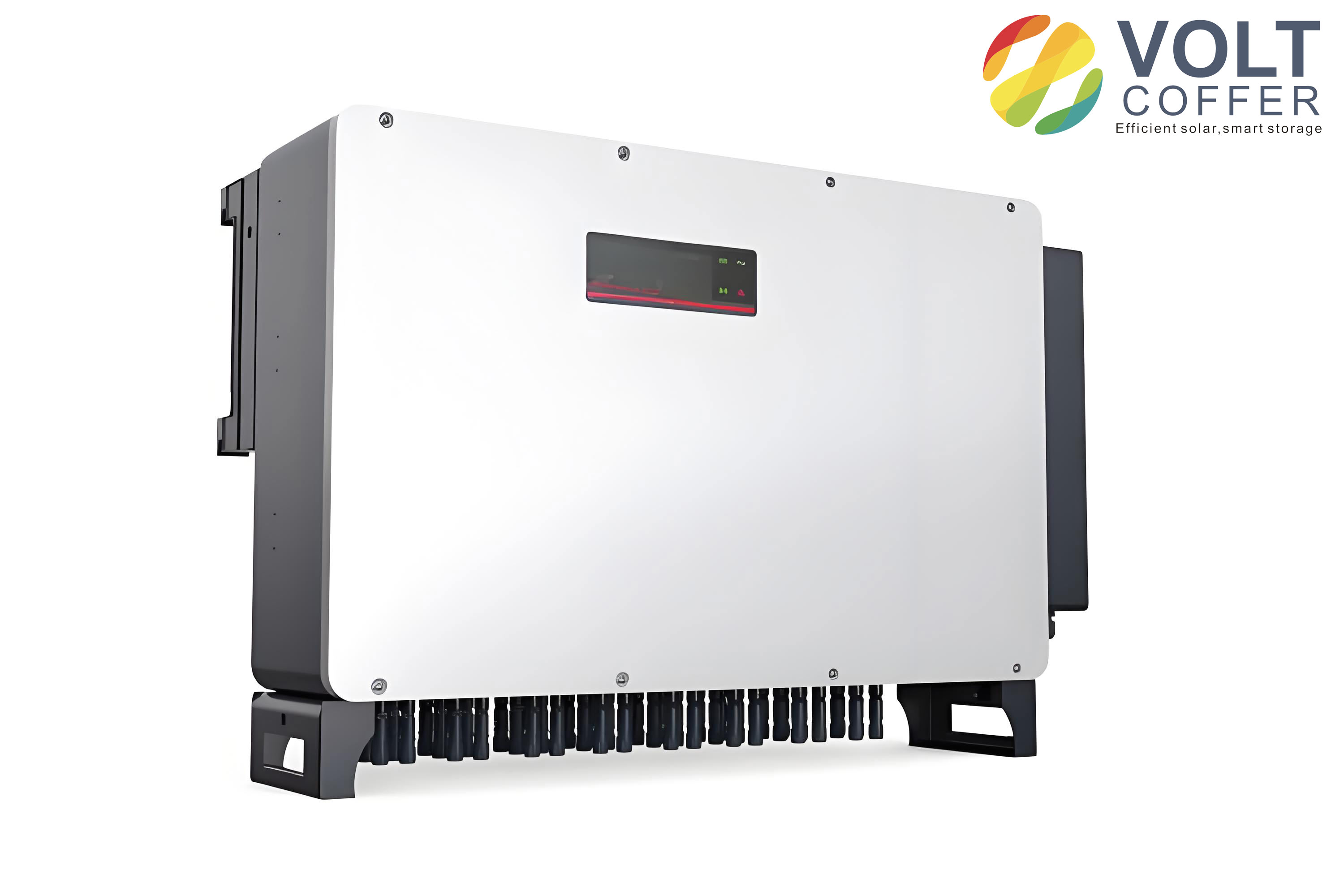
I compared the common photovoltaic system architectures before fixing the design. The centralized architecture uses many photovoltaic modules connected in series and parallel, followed by a large solar inverter. The AC-module architecture integrates a small solar inverter with each module. The string architecture connects modules in series and uses a string solar inverter. The multi-branch architecture uses several DC-DC converters and a common inverter. The master-slave architecture changes its structure dynamically according to operating conditions.
| Architecture | Typical Power Level | Advantages | Limitations |
|---|---|---|---|
| Centralized | High | Simple centralized control, low cost per watt | Poor module-level MPPT, large mismatch loss |
| AC module | Low | Module-level MPPT, easy expansion | High cost per watt, lower inverter efficiency |
| String | Medium | Reduced mismatch, good efficiency | Partial shading affects the string |
| Multi-branch | Medium to high | Independent MPPT per branch, high stability | More complex control and hardware |
| Master-slave | Medium to high | High efficiency over a wide range | Coordinated switching complexity |
For the solar inverter itself, I also reviewed isolated and non-isolated classifications. An isolated solar inverter can use a line-frequency transformer or a high-frequency transformer. The line-frequency isolated solar inverter provides galvanic isolation and safety, but it is bulky and expensive. The high-frequency isolated solar inverter reduces size and weight, but its conversion stages are more complex. A non-isolated solar inverter can be single-stage or multistage. The single-stage type requires a high DC input and has limited voltage regulation. The multistage type combines a DC-DC converter with a DC-AC inverter and offers better control freedom.
| Solar Inverter Type | Isolation | Stages | Key Features |
|---|---|---|---|
| Line-frequency isolated | Yes | DC-AC plus transformer | Safety, simple inverter control, large transformer |
| High-frequency isolated | Yes | DC-HFAC-DC-AC | Small magnetics, complex topology |
| Single-stage non-isolated | No | DC-AC | High array voltage required, compact |
| Multistage non-isolated | No | DC-DC plus DC-AC | Flexible voltage matching, good control |
I therefore adopted a multistage non-isolated solar inverter: Boost plus full bridge plus output filter. The DC-link voltage is regulated to a value above the grid voltage peak, and the full-bridge solar inverter controls the AC current. This structure allows me to separate voltage conversion from current shaping, which simplifies the control design.
Modulation Method for the Solar Inverter
I used a double-frequency sinusoidal pulse-width modulation method for the full-bridge solar inverter. In this method, one half-bridge is driven by comparing a sinusoidal modulation wave with a triangular carrier, while the other half-bridge is driven by comparing the inverted sinusoidal modulation wave with the same triangular carrier. The resulting output voltage has a switching frequency that is twice the carrier frequency, which reduces switching loss and improves harmonic performance.
Let the modulation wave be \(u_{r1}\) and the inverted modulation wave be \(u_{r2}\). Let the triangular carrier be \(u_c\). The gate signals \(u_{g1}\) and \(u_{g4}\) are complementary, and the gate signals \(u_{g2}\) and \(u_{g3}\) are complementary. The output voltage of the full bridge can be expressed as a switching function:
$$
u_o =
\begin{cases}
+u_d, & V_1 \text{ and } V_3 \text{ are on} \\
0, & V_1 \text{ and } V_4 \text{ are on, or } V_2 \text{ and } V_3 \text{ are on} \\
-u_d, & V_2 \text{ and } V_4 \text{ are on}
\end{cases}
$$
For the positive half-cycle, the active states produce \(+u_d\) or \(0\). For the negative half-cycle, the active states produce \(-u_d\) or \(0\). The average output over a switching period follows the sinusoidal reference. Because the effective switching frequency seen by the output filter is doubled, the filter can be smaller for the same harmonic attenuation.
| Modulation Feature | Effect in the Solar Inverter |
|---|---|
| Carrier frequency | Sets fundamental switching rate |
| Double-frequency update | Equivalent output ripple frequency is twice the carrier |
| Complementary gate signals | Prevents simultaneous conduction in each half-bridge |
| Dead time | Avoids shoot-through, introduces small distortion |
| Inverted modulation wave | Produces the required bipolar output voltage |
I selected a switching frequency of \(12.8\,\text{kHz}\) for the prototype. The dead time was set to \(2\,\mu\text{s}\). These values balance switching loss, harmonic content, and safe commutation. For the solar inverter, the modulation method is not only a waveform-generation issue; it also affects the current-loop bandwidth, because the current controller must be synchronized with the PWM update.
Boost Stage Modeling of the Solar Inverter
I modeled the Boost stage first because it determines the DC-link voltage available to the solar inverter. The Boost converter contains an inductor, a switch, a diode, a capacitor, and a load. In continuous conduction mode, there are two operating states: the switch is on, or the switch is off.
When the switch is on, the inductor is connected to the input source, and the capacitor supplies the load. When the switch is off, the input source and inductor deliver energy to the capacitor and load through the diode. Under steady-state conditions, the energy stored in the inductor during the on-time equals the energy released during the off-time:
$$
E I_L t_{on} = (U_o – E) I_L t_{off}
$$
Therefore, the ideal Boost voltage relation is:
$$
U_o = \frac{T}{t_{off}} E = \frac{1}{1-d} E
$$
where \(T=t_{on}+t_{off}\) and \(d=t_{on}/T\). This equation shows that the Boost converter can raise the photovoltaic voltage to the required DC-link voltage. The duty ratio must be limited so that the solar inverter does not exceed safe voltage ratings.
| Boost State | Switch | Diode | Inductor Behavior | Capacitor Behavior |
|---|---|---|---|---|
| On-state | Conducting | Blocking | Charged by input source | Supplies load |
| Off-state | Blocking | Conducting | Releases energy | Charged by source and inductor |
For dynamic modeling, I used the state-space averaging method. Let the state vector be:
$$
x =
\begin{bmatrix}
i_L \\
u_C
\end{bmatrix}
$$
During the on-state, the state equation is:
$$
\frac{d}{dt}
\begin{bmatrix}
i_L \\
u_C
\end{bmatrix}
=
\begin{bmatrix}
0 & 0 \\
0 & -\frac{1}{RC}
\end{bmatrix}
\begin{bmatrix}
i_L \\
u_C
\end{bmatrix}
+
\begin{bmatrix}
\frac{1}{L} \\
0
\end{bmatrix}
E
$$
During the off-state, the state equation is:
$$
\frac{d}{dt}
\begin{bmatrix}
i_L \\
u_C
\end{bmatrix}
=
\begin{bmatrix}
0 & -\frac{1}{L} \\
\frac{1}{C} & -\frac{1}{RC}
\end{bmatrix}
\begin{bmatrix}
i_L \\
u_C
\end{bmatrix}
+
\begin{bmatrix}
\frac{1}{L} \\
0
\end{bmatrix}
E
$$
After averaging over one switching period, I obtained:
$$
\frac{d\langle x \rangle_{T_s}}{dt} = A \langle x \rangle_{T_s} + B \langle u \rangle_{T_s}
$$
where
$$
A =
\begin{bmatrix}
0 & -\frac{1-d}{L} \\
\frac{1-d}{C} & -\frac{1}{RC}
\end{bmatrix},
\quad
B =
\begin{bmatrix}
\frac{1}{L} \\
0
\end{bmatrix}
$$
The steady-state operating point is obtained by setting the derivative to zero:
$$
X = -A^{-1} B U
$$
which gives
$$
U_C = \frac{E}{1-d},
\quad
I_L = \frac{E}{(1-d)^2 R}
$$
These expressions helped me choose the Boost inductor, DC-link capacitor, and duty-ratio limits for the solar inverter. I also used them to verify that the DC-link voltage remains above the grid voltage peak under the expected input-voltage range.
| Boost Parameter | Design Consideration |
|---|---|
| Input voltage | Must be below DC-link reference |
| Duty ratio | Limited to prevent overvoltage and instability |
| Inductor | Limits current ripple and maintains continuous conduction |
| Capacitor | Limits DC-link voltage ripple |
| Switching frequency | Trade-off between size and loss |
Inverter Stage Modeling of the Solar Inverter
For the inverter stage, I considered the full bridge and the output filter. The bridge output voltage is \(u_a\), and the grid voltage is \(u_o\). The current flowing through the filter inductor is \(i_L\). Applying Kirchhoff’s voltage law gives:
$$
u_a = L \frac{di_L}{dt} + R i_L + u_o
$$
Rearranging:
$$
u_a – u_o = L \frac{di_L}{dt} + R i_L
$$
Taking the Laplace transform with zero initial conditions:
$$
U_a(s) – U_o(s) = (Ls + R) I_L(s)
$$
Thus the transfer function from the voltage difference to the inductor current is:
$$
G_i(s) = \frac{I_L(s)}{U_a(s)-U_o(s)} = \frac{1}{Ls+R}
$$
If the PWM inverter is treated as a proportional gain \(K_{\text{PWM}}\), the open-loop transfer function of the current loop becomes:
$$
G_{\text{open}}(s) = \frac{K_{\text{PWM}}}{Ls+R}
$$
This first-order model ignores switch nonlinearities, dead time, and sensor delay. Even so, it is useful for tuning the PI current regulator. In my design, I used the model to select a current-loop bandwidth well below the switching frequency but high enough to track the sinusoidal reference.
| Inverter Stage Element | Modeling Role |
|---|---|
| Full bridge | Produces switched voltage \(u_a\) |
| Filter inductor | Smooths current and determines current dynamics |
| Equivalent resistance | Represents losses and damping |
| Grid voltage | Disturbance in the current loop |
| PWM block | Approximated as a gain for control design |
Virtual Space Vector Principle for the Solar Inverter
The control challenge of a single-phase solar inverter is that only one AC quantity is measured. In a three-phase system, coordinate transformation naturally uses three phases and produces two orthogonal components. In a single-phase solar inverter, I need two orthogonal components to perform Park transformation. Therefore, I construct a virtual orthogonal quantity. This is the core of the virtual space vector method.
Let the measured grid-side current of the solar inverter be:
$$
i_\alpha = I_m \cos(\omega t + \phi)
$$
I generate a virtual current \(i_\beta\) that has the same amplitude and frequency but is shifted by \(90^\circ\):
$$
i_\beta = I_m \sin(\omega t + \phi)
$$
Now \(i_\alpha\) and \(i_\beta\) form a two-phase stationary orthogonal pair. I apply the Park transformation:
$$
\begin{bmatrix}
i_d \\
i_q
\end{bmatrix}
=
\begin{bmatrix}
\cos\theta & \sin\theta \\
-\sin\theta & \cos\theta
\end{bmatrix}
\begin{bmatrix}
i_\alpha \\
i_\beta
\end{bmatrix}
$$
If the estimated angle \(\theta\) is equal to the actual grid angle, then \(i_d\) and \(i_q\) become DC quantities. For a current-controlled solar inverter, \(i_d\) represents the active current component, and \(i_q\) represents the reactive current component. I can regulate them with PI controllers, which have zero steady-state error for DC signals.
The inverse transformation is:
$$
\begin{bmatrix}
i_\alpha^* \\
i_\beta^*
\end{bmatrix}
=
\begin{bmatrix}
\cos\theta & -\sin\theta \\
\sin\theta & \cos\theta
\end{bmatrix}
\begin{bmatrix}
i_d^* \\
i_q^*
\end{bmatrix}
$$
The output \(i_\alpha^*\) is used as the modulation reference for the solar inverter. The virtual component \(i_\beta^*\) is not directly needed for a single-phase output, but it is necessary for the internal coordinate transformation. In this way, the single-phase solar inverter is controlled as if it were a two-axis system.
| Control Quantity | Physical Meaning in the Solar Inverter |
|---|---|
| \(i_\alpha\) | Measured grid-side AC current |
| \(i_\beta\) | Virtual orthogonal current generated by Hilbert transform |
| \(i_d\) | Active current component |
| \(i_q\) | Reactive current component |
| \(\theta\) | Grid phase angle from the PLL |
Hilbert Transform for Virtual Vector Generation
I used the Hilbert transform to generate the virtual orthogonal signal for the solar inverter. For a continuous-time signal \(x(t)\), the Hilbert transform is defined as:
$$
\hat{x}(t) = H\{x(t)\} = \frac{1}{\pi} \int_{-\infty}^{\infty} \frac{x(\tau)}{t-\tau} d\tau
$$
Equivalently, it can be written as a convolution:
$$
\hat{x}(t) = x(t) * \frac{1}{\pi t}
$$
The frequency response of the Hilbert transformer is:
$$
H(j\omega) = -j\,\operatorname{sgn}(\omega)
$$
Its magnitude is unity for all nonzero frequencies:
$$
|H(j\omega)| = 1
$$
Its phase is \(-\pi/2\) for positive frequencies and \(+\pi/2\) for negative frequencies. Therefore, a sinusoidal signal is shifted by \(90^\circ\) while its amplitude is preserved. This property is exactly what I need to build the virtual vector for the solar inverter.
For digital implementation, I used the discrete Hilbert transform based on the discrete Fourier transform. For a sequence \(x(n)\) of length \(N\), I compute its DFT \(X(k)\). Then I define:
$$
Z(k) =
\begin{cases}
X(0), & k=0 \\
2X(k), & 1 \le k \le \frac{N}{2}-1 \\
X(N/2), & k=\frac{N}{2} \\
0, & \frac{N}{2}+1 \le k \le N-1
\end{cases}
$$
Then I apply the inverse DFT to \(Z(k)\). The result is the analytic signal:
$$
z(n) = x(n) + j\hat{x}(n)
$$
The imaginary part \(\hat{x}(n)\) is the Hilbert-transformed sequence. In my DSP software, I used this method to produce the orthogonal current for the solar inverter. I verified the algorithm with a 16-point test sequence. The input and output sequences confirmed a \(90^\circ\) phase shift.
| \(n\) | Input \(x(n)\) | Hilbert Output \(\hat{x}(n)\) |
|---|---|---|
| 0 | 0.0000 | -1.0000 |
| 1 | 0.3827 | -0.9238 |
| 2 | 0.7071 | -0.7071 |
| 3 | 0.9239 | -0.3826 |
| 4 | 1.0000 | 0.0000 |
| 5 | 0.9239 | 0.3826 |
| 6 | 0.7071 | 0.7071 |
| 7 | 0.3827 | 0.9238 |
| 8 | 0.0000 | 1.0000 |
| 9 | -0.3827 | 0.9238 |
| 10 | -0.7071 | 0.7071 |
| 11 | -0.9239 | 0.3826 |
| 12 | -1.0000 | 0.0000 |
| 13 | -0.9239 | -0.3826 |
| 14 | -0.7071 | -0.7071 |
| 15 | -0.3827 | -0.9238 |
The Hilbert transform is attractive for the solar inverter because it provides a clean quadrature signal without an additional phase-locked oscillator. However, it requires computation, so I placed it inside the PWM interrupt and optimized the DFT/IDFT routine for the fixed sequence length. I also verified that the amplitude of the virtual signal matches the measured current amplitude closely enough for current control.
Phase-Locked Loop for the Solar Inverter
The virtual space vector method requires an accurate grid angle. I used a single synchronous reference frame software phase-locked loop, often abbreviated SSRF-SPLL. The measured grid voltage and its Hilbert-transformed virtual voltage are transformed into the \(dq\) frame. The \(q\)-axis voltage is driven to zero by a PI regulator. The output of the PI regulator is added to the nominal grid frequency to produce the estimated angular frequency, which is then integrated to obtain the phase angle.
Let the grid voltage be \(V\) and the estimated angle be \(\theta^*\). The \(dq\) components are:
$$
v_d = V \cos(\theta – \theta^*)
$$
$$
v_q = V \sin(\theta – \theta^*)
$$
When the PLL is locked, \(\theta^* \approx \theta\), so \(v_q \approx 0\) and \(v_d \approx V\). The PI controller for the PLL can be written as:
$$
\omega^* = \omega_{ff} + K_{p,\text{PLL}} v_q + K_{i,\text{PLL}} \int v_q dt
$$
$$
\theta^* = \int \omega^* dt
$$
The feed-forward term \(\omega_{ff}\) is the nominal grid angular frequency. The PI regulator eliminates the phase error. For the solar inverter, this angle is used in both the forward Park transformation and the inverse Park transformation.
| PLL Variable | Role in the Solar Inverter |
|---|---|
| \(v_\alpha\) | Measured grid voltage |
| \(v_\beta\) | Virtual orthogonal grid voltage |
| \(v_d\) | Direct-axis voltage |
| \(v_q\) | Quadrature-axis voltage, regulated to zero |
| \(\theta^*\) | Phase angle used by Park and inverse Park transformations |
| \(\omega^*\) | Estimated angular frequency |
I tested the PLL under a grid voltage amplitude change. The PLL continued to track the grid angle, and the output angle increased from \(0\) to \(2\pi\) within each \(0.02\,\text{s}\) period. This confirmed that the solar inverter could maintain synchronization even when the grid voltage was not constant.
Current Loop and PI Regulation for the Solar Inverter
For the current loop, I used PI regulators in the \(dq\) frame. Because \(i_d\) and \(i_q\) are DC quantities under locked conditions, the PI regulators can achieve zero steady-state error. The reference \(i_d^*\) sets the active current, while \(i_q^*\) sets the reactive current. In my grid-connected solar inverter, I usually set \(i_q^*=0\) to inject current at unity power factor, although the structure allows reactive power control if needed.
The continuous PI control law is:
$$
u(t) = K_p e(t) + K_i \int_0^t e(\tau) d\tau + u_0
$$
For digital implementation, I used the discrete form:
$$
u_k = u_{k-1} + K_p(e_k – e_{k-1}) + K_i e_k
$$
To prevent integral windup, I limited the output and used an anti-windup correction. The algorithm can be summarized as:
$$
u_k = u_{k-1} + K_p(e_k – e_{k-1}) + K_i e_k
$$
$$
u_k =
\begin{cases}
u_{\max}, & u_k > u_{\max} \\
u_{\min}, & u_k < u_{\min} \\
u_k, & \text{otherwise}
\end{cases}
$$
When the output saturates, the integral term is adjusted so that the controller does not accumulate excessive error. This is important in the solar inverter because the current reference can change rapidly during grid voltage disturbances or during startup.
| Controller | Input | Output | Purpose |
|---|---|---|---|
| Current PI for \(i_d\) | \(i_d^* – i_d\) | \(u_d^*\) | Active current regulation |
| Current PI for \(i_q\) | \(i_q^* – i_q\) | \(u_q^*\) | Reactive current regulation |
| PLL PI | \(v_q\) | \(\omega^*\) | Grid synchronization |
| Voltage outer loop, optional | \(u_{dc}^* – u_{dc}\) | \(i_d^*\) | DC-link voltage regulation |
I tuned the current PI gains so that the current response was fast but not oscillatory. The current loop bandwidth was set much lower than the switching frequency to avoid interaction with PWM ripple. The final current waveform tracked the grid voltage with low phase error and low harmonic distortion.
Simulation Study of the Solar Inverter
I built a simulation model of the solar inverter to verify the control strategy before hardware implementation. The model included the main power circuit, the Boost stage, the full-bridge inverter, the output filter, the virtual vector generator, the PLL, the coordinate transformations, the PI regulators, and the PWM generation block. I used a programmable voltage source to emulate the grid so that I could observe the dynamic response of the solar inverter.
| Simulation Parameter | Value |
|---|---|
| Grid nominal voltage | 220 V RMS |
| Grid frequency | 50 Hz |
| DC-link voltage | 400 V |
| Switching frequency | 12.8 kHz |
| Current reference \(i_d^*\) | 20 A |
| Reactive reference \(i_q^*\) | 0 A |
| Grid voltage step | 38 V between 0.3 s and 0.5 s |
| Transformer ratio for virtual test | 2 |
The simulation results showed that the Hilbert transform produced a virtual voltage vector shifted by \(90^\circ\) from the measured grid voltage. The PLL output angle tracked the grid voltage period accurately. After the Park transformation, the current components became DC quantities. The \(d\)-axis current settled near \(20\,\text{A}\), and the \(q\)-axis current settled near \(0\,\text{A}\). The PI regulators produced smooth outputs, and the inverse Park transformation generated a sinusoidal modulation reference for the PWM block.
| Simulation Stage | Expected Behavior | Observed Result |
|---|---|---|
| Hilbert transform | 90 degree phase shift | Virtual vector orthogonal to measured quantity |
| PLL | Track grid angle | Angle followed grid period and changes |
| Park transform | AC to DC | \(i_d\) and \(i_q\) became smooth DC |
| PI current loop | Zero steady-state error | \(i_d \approx 20\,\text{A}\), \(i_q \approx 0\,\text{A}\) |
| Inverse Park transform | DC to AC reference | Sinusoidal modulation signal produced |
| PWM and filter | Grid current tracking | Output current followed grid voltage |
When the grid voltage amplitude changed between \(0.3\,\text{s}\) and \(0.5\,\text{s}\), the current remained stable at approximately \(20\,\text{A}\). This demonstrated that the current loop rejected the grid voltage disturbance and that the virtual space vector method was effective for the single-phase solar inverter. The output current had low ripple and fast tracking, which validated the control strategy.
Hardware Design of the Solar Inverter
After simulation, I designed and built a prototype solar inverter. The hardware included a switch-mode power supply, a main control board, driver circuits, sampling circuits, a Boost power stage, a full-bridge inverter stage, and an output filter. The main controller was a fixed-point DSP. Because the DSP does not support floating-point arithmetic natively, I used fixed-point representation for the control variables and carefully scaled the current, voltage, and angle signals.
| Hardware Block | Function in the Solar Inverter |
|---|---|
| Switch-mode power supply | Provides regulated DC bias for control and driver circuits |
| Main control board | Executes ADC sampling, PLL, Hilbert transform, Park transform, PI control, and PWM generation |
| Driver circuit | Amplifies DSP PWM signals to drive the power switches |
| Boost stage | Raises photovoltaic voltage to the DC-link level |
| Full-bridge inverter | Converts DC-link power to AC current |
| Output filter | Attenuates high-frequency harmonics before grid connection |
| Voltage and current sensors | Provide feedback for PLL and current control |
For the DC voltage sampling circuit, I used a resistor divider followed by a voltage follower and an isolation amplifier. The divider scaled the high DC voltage down to the DSP ADC range. A clamping circuit limited the signal to a safe range. For the AC voltage sampling circuit, I used a voltage transformer and an operational amplifier. Because the AC signal is bipolar and the ADC accepts only positive voltages, I added a level-shifting circuit. The ADC input after level shifting can be written as:
$$
u_{\text{ADC}} = \frac{u’ R_{74} + V_{CC} R_{69}}{R_{74}+R_{69}}
$$
For the AC current sampling circuit, I used a Hall-effect current sensor. The sensor output was conditioned by a voltage follower, level shifter, and clamp. The final signal was connected to the ADC channel. This arrangement allowed the solar inverter to measure the grid-side current in real time.
| Signal | Sensor Type | Conditioning | ADC Purpose |
|---|---|---|---|
| DC-link voltage | Resistor divider | Follower, isolation, clamp | Boost and protection |
| Grid voltage | Voltage transformer | Amplifier, level shift, clamp | PLL and synchronization |
| Grid current | Hall-effect sensor | Follower, level shift, clamp | Current loop |
Software Design of the Solar Inverter
I organized the solar inverter software using a foreground-background structure. The main loop performs initialization and non-time-critical tasks. The PWM interrupt performs the real-time control tasks. This separation ensures that current sampling, virtual vector generation, coordinate transformation, PI regulation, and PWM update occur at a fixed rate.
| Software Module | Execution Context | Function |
|---|---|---|
| System initialization | Main loop | Configure clocks, GPIO, ADC, PWM, and interrupts |
| ADC sampling | PWM interrupt | Read DC voltage, grid voltage, and grid current |
| Hilbert transform | PWM interrupt | Generate virtual orthogonal current |
| Software PLL | PWM interrupt | Estimate grid phase angle |
| Park transform | PWM interrupt | Convert \(\alpha\beta\) to \(dq\) |
| PI current control | PWM interrupt | Regulate \(i_d\) and \(i_q\) |
| Inverse Park transform | PWM interrupt | Generate sinusoidal modulation reference |
| PWM update | PWM interrupt | Write compare registers for the full bridge |
The main program initializes the system and then enters an infinite loop. The PWM interrupt is the main real-time event. In the interrupt, the ADC results are read, the Hilbert transform creates the virtual current, the software PLL updates the angle, the Park transformation produces \(i_d\) and \(i_q\), the PI regulators compute the voltage references, the inverse Park transformation returns the reference to the stationary frame, and the PWM compare registers are updated.
The startup sequence of the solar inverter is also important. When the photovoltaic voltage is sufficient, the Boost stage begins to raise the DC-link voltage. The controller checks whether the DC-link voltage exceeds the minimum required value and whether the grid voltage amplitude, frequency, and phase are within limits. If these conditions are satisfied, the PLL locks, the PWM is enabled, and the relay connects the solar inverter to the grid. The current loop then regulates the injected current.
| Startup Condition | Action in the Solar Inverter |
|---|---|
| PV voltage acceptable | Enable Boost stage |
| DC-link voltage acceptable | Prepare inverter for synchronization |
| Grid voltage and frequency acceptable | Run PLL and check synchronization |
| PLL locked | Enable PWM and close current loop |
| Current tracked | Close grid relay |
| Fault detected | Disable PWM and open relay |
Experimental Results of the Solar Inverter
I tested the prototype solar inverter with a photovoltaic simulator and an oscilloscope. The input voltage was set to approximately \(200\,\text{V}\). The Boost stage raised the DC-link voltage to about \(400\,\text{V}\). The grid voltage was \(220\,\text{V}\) RMS at \(50\,\text{Hz}\). The switching frequency was \(12.8\,\text{kHz}\), and the dead time was \(2\,\mu\text{s}\). The prototype was rated for \(3\,\text{kW}\).
| Experimental Parameter | Value |
|---|---|
| Rated power | 3 kW |
| Input DC voltage | 200 V |
| DC-link voltage | 400 V |
| Grid voltage | 220 V RMS |
| Grid frequency | 50 Hz |
| Switching frequency | 12.8 kHz |
| Dead time | 2 microseconds |
| Output voltage peak | 311 V |
| Output current peak | 20 A |
| Phase error | Less than 1 percent |
The double-frequency SPWM gate signals showed complementary operation in each half-bridge. The upper and lower switches of each leg never conducted simultaneously. The output voltage and grid voltage were nearly in phase. The measured phase error was less than 1 percent, and the output voltage remained stable. The output current followed the grid voltage with low ripple and a stable sinusoidal shape.
| Observed Quantity | Result | Interpretation |
|---|---|---|
| Gate signals | Complementary with dead time | Safe full-bridge operation |
| PLL angle | Tracked grid period | Synchronization achieved |
| Output voltage | 311 V peak | Matches grid voltage amplitude |
| Output current | 20 A peak | Current loop regulated active current |
| Phase error | Less than 1 percent | Good grid synchronization |
| Dynamic response | Stable under voltage step | Effective disturbance rejection |
I also observed the behavior during a grid voltage amplitude change. In simulation, the voltage step occurred between \(0.3\,\text{s}\) and \(0.5\,\text{s}\). The current remained stable at \(20\,\text{A}\). In the prototype, the current loop also maintained stable operation when the grid voltage varied within the tested range. This confirmed that the virtual space vector method improves the dynamic performance of the solar inverter.
Protection and Grid Compliance of the Solar Inverter
I included basic protection functions in the solar inverter. The DC voltage was monitored for undervoltage and overvoltage. The AC current was monitored for overcurrent and short circuit. The grid voltage was monitored for overvoltage, undervoltage, overfrequency, and underfrequency. When a fault was detected, the DSP disabled the PWM signals and opened the grid relay.
| Protection Function | Detection Signal | Action |
|---|---|---|
| DC undervoltage | DC-link voltage | Disable Boost and inverter |
| DC overvoltage | DC-link voltage | Disable Boost, open relay |
| AC overcurrent | Grid current | Disable PWM, open relay |
| AC overvoltage | Grid voltage | Disconnect from grid |
| AC undervoltage | Grid voltage | Disconnect from grid |
| Overfrequency | PLL frequency | Disconnect from grid |
| Underfrequency | PLL frequency | Disconnect from grid |
| Islanding | Grid state estimation | Future work for the solar inverter |
The prototype did not include a complete anti-islanding function. I consider this a limitation. In a practical grid-connected solar inverter, islanding detection is necessary because the inverter must not energize a disconnected grid section. Future work should add active or passive islanding detection and verify it under grid fault conditions.
Discussion of the Virtual Space Vector Solar Inverter
I found that the virtual space vector method gives the single-phase solar inverter a control structure similar to a three-phase inverter. The Hilbert transform provides the missing orthogonal axis, and the PLL provides the rotating angle. The current controller then operates on DC quantities, which makes PI tuning straightforward and improves steady-state accuracy. The solar inverter can regulate active and reactive current independently, although I set the reactive reference to zero in the tested unity-power-factor case.
The Boost stage is essential for voltage matching. It allows the solar inverter to operate with a lower photovoltaic input voltage while maintaining a DC link above the grid peak. The state-space averaged model provides a clear design equation for the duty ratio and component selection. The full-bridge inverter with double-frequency SPWM reduces harmonic current and switching loss. The output filter attenuates the remaining high-frequency components.
| Design Aspect | Benefit for the Solar Inverter | Trade-off |
|---|---|---|
| Boost plus full bridge | Flexible voltage matching and current control | More components and control complexity |
| Double-frequency SPWM | Lower switching loss and smaller filter | Requires complementary modulation logic |
| Virtual space vector control | DC-style PI regulation and fast response | Requires Hilbert transform and PLL |
| Software PLL | Accurate synchronization without extra hardware | Computational load in the interrupt |
| Fixed-point DSP | Low cost and deterministic timing | Scaling and quantization care |
I also noted several practical issues. Dead time introduces low-order distortion in the output current. Sensor offset and gain errors affect the virtual vector amplitude and the PLL angle. Fixed-point arithmetic requires careful scaling to avoid overflow in the PI regulators and the Hilbert transform. The PWM interrupt execution time must remain below the switching period. I addressed these issues by using clamped ADC signals, calibrated offsets, limited PI outputs, and optimized code.
Comparison with Alternative Control Methods for the Solar Inverter
I compared the virtual space vector current control with other common methods. A simple PI current regulator in the stationary frame cannot eliminate sinusoidal steady-state error without an additional resonant term. A proportional-resonant controller can track a sinusoidal reference accurately, but its tuning is frequency sensitive. Hysteresis current control has fast response but variable switching frequency and high harmonic content. Model predictive control can be fast, but it requires more computation and an accurate model.
| Control Method | Steady-State Accuracy | Dynamic Response | Implementation Complexity |
|---|---|---|---|
| Stationary PI | Limited for AC reference | Moderate | Low |
| Proportional-resonant | High at selected frequency | Good | Moderate |
| Hysteresis | Depends on band | Fast | Low |
| Virtual space vector with PI | High due to DC regulation | Fast | Moderate |
| Model predictive | High with accurate model | Very fast | High |
I selected the virtual space vector method because it uses the well-known \(dq\) PI framework, achieves zero steady-state error for DC quantities, and provides a clear path to reactive power control. For a single-phase solar inverter, the main cost is the generation of the virtual orthogonal signal. The Hilbert transform proved to be a reliable method for this purpose.
Key Equations of the Solar Inverter Control
The following equations summarize the main control relationships I used in the solar inverter.
Boost voltage gain:
$$
U_o = \frac{1}{1-d}E
$$
Boost steady-state inductor current:
$$
I_L = \frac{E}{(1-d)^2 R}
$$
Inverter current dynamics:
$$
u_a – u_o = L \frac{di_L}{dt} + R i_L
$$
Current transfer function:
$$
G_i(s) = \frac{1}{Ls+R}
$$
Hilbert transform:
$$
\hat{x}(t) = \frac{1}{\pi} \int_{-\infty}^{\infty} \frac{x(\tau)}{t-\tau} d\tau
$$
Park transformation:
$$
\begin{bmatrix}
i_d \\
i_q
\end{bmatrix}
=
\begin{bmatrix}
\cos\theta & \sin\theta \\
-\sin\theta & \cos\theta
\end{bmatrix}
\begin{bmatrix}
i_\alpha \\
i_\beta
\end{bmatrix}
$$
Inverse Park transformation:
$$
\begin{bmatrix}
i_\alpha^* \\
i_\beta^*
\end{bmatrix}
=
\begin{bmatrix}
\cos\theta & -\sin\theta \\
\sin\theta & \cos\theta
\end{bmatrix}
\begin{bmatrix}
i_d^* \\
i_q^*
\end{bmatrix}
$$
PLL error:
$$
v_q = V\sin(\theta-\theta^*)
$$
PI regulator:
$$
u(t) = K_p e(t) + K_i \int_0^t e(\tau)d\tau
$$
Discrete PI regulator:
$$
u_k = u_{k-1} + K_p(e_k-e_{k-1}) + K_i e_k
$$
| Equation Group | Use in the Solar Inverter |
|---|---|
| Boost gain | Set DC-link voltage above grid peak |
| Boost state-space model | Design inductor and capacitor |
| Inverter current dynamics | Tune current PI regulator |
| Hilbert transform | Create virtual orthogonal current |
| Park and inverse Park | Convert between AC and DC control frames |
| PLL error | Lock grid phase and frequency |
| PI equations | Regulate current and PLL |
Design Iteration and Practical Observations
I iterated the design several times. The first step was to verify the Boost stage independently. I checked that the duty ratio was limited and that the DC-link voltage remained stable under load. The second step was to verify the full-bridge inverter with open-loop PWM. I observed the gate signals and the output voltage before closing the current loop. The third step was to verify the PLL in open loop. I confirmed that the angle increased linearly with time and reset every grid period. The fourth step was to verify the Hilbert transform. I compared the measured current with the virtual current and confirmed the \(90^\circ\) phase difference. The fifth step was to close the current loop and observe the grid current.
| Commissioning Step | Goal | Result |
|---|---|---|
| Boost open-loop | Verify voltage gain | DC-link reached target |
| Inverter open-loop | Verify PWM and dead time | Complementary gate signals observed |
| PLL open-loop | Verify phase tracking | Angle followed grid period |
| Hilbert transform | Verify quadrature signal | Virtual current shifted by 90 degrees |
| Current closed-loop | Verify grid current control | Current tracked reference |
| Grid disturbance test | Verify dynamic response | Current remained stable |
During commissioning, I found that ADC offset calibration was important. A small offset in the current sensor produced a DC component in the \(dq\) frame, which caused the current reference to shift. I corrected this by sampling zero-current offset at startup and subtracting it in software. I also found that the PLL gains must be low enough to reject grid harmonics but high enough to track frequency changes. The final gains provided a good balance.
Experimental Waveform Interpretation
The experimental waveforms showed that the solar inverter produced a sinusoidal output current synchronized with the grid voltage. The output voltage and grid voltage were almost coincident. The current waveform had low ripple because the output filter attenuated the switching harmonics. The current amplitude was about \(20\,\text{A}\) peak, and the voltage amplitude was about \(311\,\text{V}\) peak. The phase error was less than 1 percent.
I also examined the double-frequency SPWM behavior. The gate signals alternated according to the sinusoidal reference and the triangular carrier. The effective switching frequency at the output was twice the carrier frequency, which reduced the harmonic content. The dead time prevented shoot-through, although it introduced a small amount of zero-crossing distortion. The current loop compensated for most of this distortion.
| Waveform | Observation | Conclusion |
|---|---|---|
| Gate signals | Complementary with dead time | Safe commutation |
| Output voltage | Stable sinusoidal shape | Inverter modulation correct |
| Grid voltage | Aligned with output voltage | PLL synchronization correct |
| Output current | Stable and smooth | Current loop effective |
| Current under voltage step | Remained near 20 A | Good disturbance rejection |
Conclusion of My Study
I designed, simulated, built, and tested a single-phase grid-connected solar inverter based on virtual space vector control. The solar inverter uses a Boost stage, a full-bridge inverter, and an output filter. The modulation method is double-frequency SPWM. The control strategy uses Hilbert transform to generate a virtual orthogonal current, a software PLL to estimate the grid angle, Park and inverse Park transformations to work in the \(dq\) frame, and PI regulators to control active and reactive current.
My main conclusions are as follows. First, the virtual space vector method allows a single-phase solar inverter to use DC-style PI current regulation with zero steady-state error. Second, the Hilbert transform provides a reliable \(90^\circ\) phase shift for the virtual vector. Third, the software PLL accurately tracks the grid angle even when the grid voltage amplitude changes. Fourth, the Boost stage successfully raises the photovoltaic voltage to the required DC-link level. Fifth, the double-frequency SPWM reduces switching loss and improves harmonic performance. Sixth, the experimental prototype achieved stable grid current, good phase alignment, and robust dynamic behavior.
The solar inverter prototype met the basic grid-connection requirements under the tested conditions. The current waveform was stable, the phase error was small, and the system responded well to grid voltage changes. The work confirms that virtual space vector control is a practical and effective method for a single-phase solar inverter.
Future improvements should include complete islanding detection, more advanced grid-voltage feedforward, adaptive PLL gains, harmonic compensation, and a full thermal and reliability assessment. These additions would make the solar inverter more robust under abnormal grid conditions and more suitable for large-scale deployment. Even with these future tasks, the present study demonstrates that the virtual space vector solar inverter is a strong candidate for high-performance single-phase photovoltaic grid connection.