
Solar photovoltaic (PV) capacity has expanded rapidly over the past decade, and solar inverters have become indispensable interfaces between PV arrays and the power grid. Among all components in a solar inverter, the insulated-gate bipolar transistor (IGBT) module is recognized as one of the most failure-prone parts. The junction temperature of IGBT modules fluctuates because of intermittent solar irradiance and changing ambient temperature. Since the materials inside an IGBT module have mismatched coefficients of thermal expansion, temperature swings cause cyclic mechanical stress between adjacent layers. This stress gradually accumulates and eventually leads to solder fatigue or bond-wire lift-off. Consequently, evaluating the lifetime of IGBT modules and developing effective thermal management strategies are crucial to improve the reliability and cost-effectiveness of solar inverters.
In this work, we present a comprehensive framework for the lifetime evaluation of IGBT modules in solar inverters and a corresponding lifetime enhancement strategy. We first propose a numerical junction temperature estimation method based on the power loss model and a one-dimensional Foster thermal network. Then we apply the method to a one-year mission profile and extract thermal cycles using rainflow counting. The lifetime consumption is calculated with the Bayerer lifetime model and Miner’s rule. We also quantify the impact of parameter uncertainty using Monte Carlo simulation. Based on the lifetime evaluation results, we develop a thermal management control strategy that determines the junction temperature threshold, the operating region, and the switching frequency adjustment. To maximize the benefit of each thermal management action, we introduce a benefit-cost ratio (BCR) as a quantitative optimization index. Experimental and case studies confirm the effectiveness of the proposed strategy.
1. Junction Temperature Estimation in Solar Inverters
1.1 System configuration and PV array model
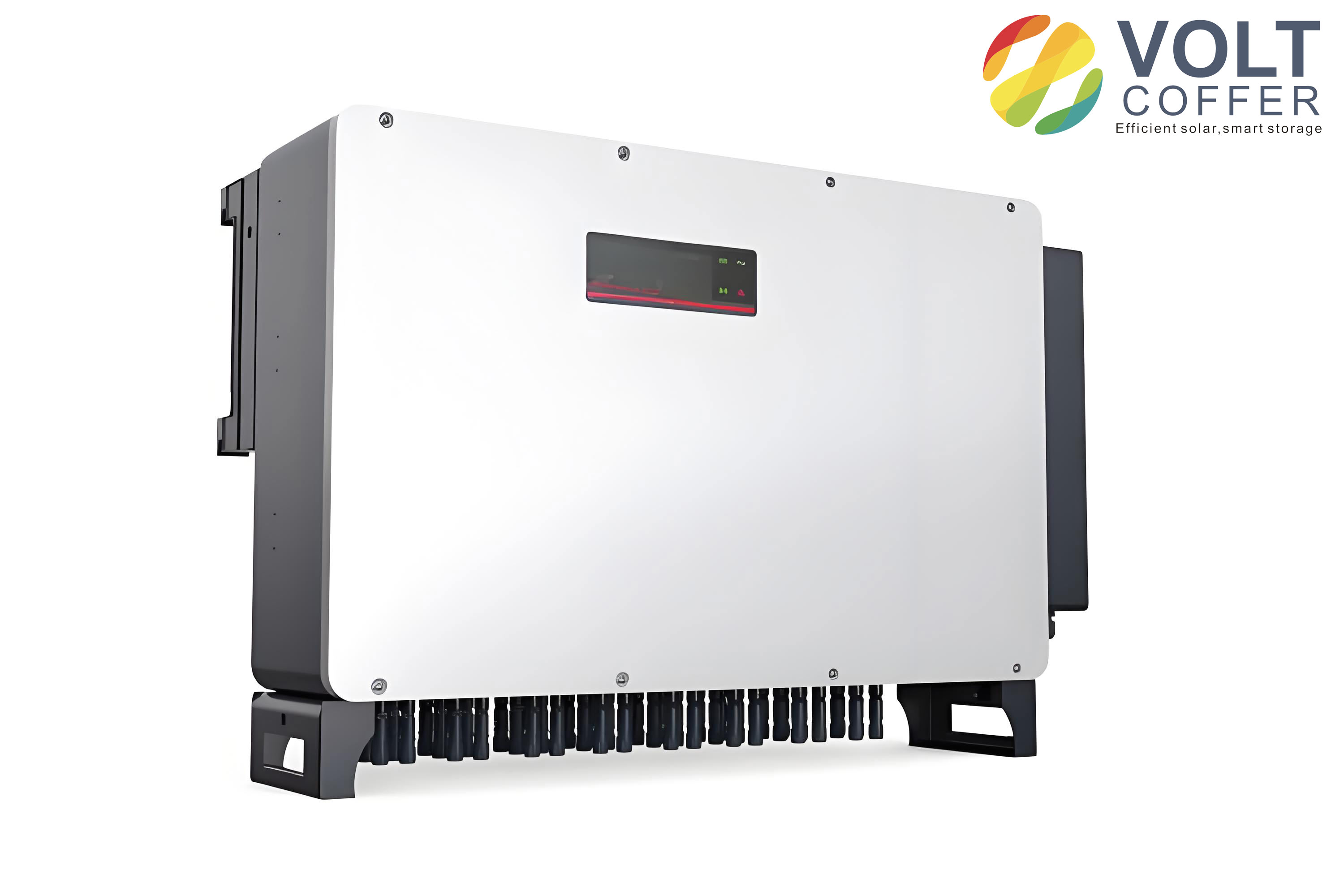
The study focuses on a three-phase single-stage grid-connected solar inverter. The system consists of a PV array, a DC-link capacitor, a three-phase inverter, an L filter, and the grid. The inverter parameters used in this work are listed in Table 1.
| Parameter | Value |
|---|---|
| Rated capacity (MW) | 1.0 |
| Rated frequency (Hz) | 50 |
| DC-link capacitance (μF) | 5000 |
| Filter inductance (μH) | 300 |
| Output voltage (V, rms) | 480 |
| IGBT switching frequency (Hz) | 3000 |
| Maximum DC-link voltage (V) | 1000 |
According to the irradiance level, the PV inverter operates in three regions. When the irradiance is below the minimum threshold \(S_{\mathrm{min}}\), the inverter is in stand-by mode. When the irradiance is between \(S_{\mathrm{min}}\) and the rated threshold \(S_{\mathrm{nom}}\), the inverter tracks the maximum power point (MPPT). When the irradiance exceeds \(S_{\mathrm{nom}}\), the inverter operates under constant power control. The output power is expressed as:
$$
P =
\begin{cases}
0, & S < S_{\mathrm{min}} \\
P_{\mathrm{mppt}}, & S_{\mathrm{min}} \le S < S_{\mathrm{nom}} \\
P_{\mathrm{nom}}, & S \ge S_{\mathrm{nom}}
\end{cases}
\tag{1}
$$
To build the PV array model, we use the datasheet characteristics of a commercial 65 W multi-crystalline module. The key electrical parameters at standard test conditions are given in Table 2. A lookup table is constructed from the current-voltage (\(I\)-\(V\)) curves at different irradiance and ambient temperature values. The PV array is formed by series and parallel connections of these modules, and its maximum output power is obtained by searching the peak of the \(P\)-\(V\) curve.
| Parameter | Value |
|---|---|
| Maximum power \(P_{\mathrm{max}}\) (W) | 65 |
| Voltage at MPP \(V_{\mathrm{mpp}}\) (V) | 17.6 |
| Current at MPP \(I_{\mathrm{mpp}}\) (A) | 3.69 |
| Short-circuit current \(I_{\mathrm{sc}}\) (A) | 3.99 |
| Open-circuit voltage \(V_{\mathrm{oc}}\) (V) | 21.7 |
| Module efficiency (%) | 12.1 |
1.2 Power loss model of the IGBT module
The IGBT module considered in this work is a half-bridge module with a rated current of 1000 A and a voltage rating of 1700 V. The total loss of the IGBT consists of conduction loss and switching loss. The conduction loss in the \(k\)-th switching cycle is calculated as:
$$
P_{\mathrm{cond}}^{(k)} = \left[ \left(a_0 T_{tj}^{(k-1)} + a_1\right) I_c^{(k)} + \left(b_0 T_{tj}^{(k-1)} + b_1\right) \right] I_c^{(k)} D^{(k)}
\tag{2}
$$
where \(T_{tj}^{(k-1)}\) is the IGBT junction temperature in the previous switching cycle, \(I_c^{(k)}\) is the collector current, and \(D^{(k)}\) is the duty cycle. The coefficients \(a_0\), \(a_1\), \(b_0\), and \(b_1\) are obtained by linear fitting of the output characteristics from the datasheet.
The switching loss is expressed as:
$$
P_{\mathrm{sw}}^{(k)} = \left[ a_{\mathrm{sw}}\left(I_c^{(k)}\right)^3 + b_{\mathrm{sw}}\left(I_c^{(k)}\right)^2 + c_{\mathrm{sw}} I_c^{(k)} \right] \frac{U_{\mathrm{dc}}}{U_{\mathrm{rated}}} f_{\mathrm{sw}} \left(d_0 T_{tj}^{(k-1)} + d_1\right)
\tag{3}
$$
where \(a_{\mathrm{sw}}\), \(b_{\mathrm{sw}}\), and \(c_{\mathrm{sw}}\) are current-dependent fitting coefficients, \(d_0\) and \(d_1\) are temperature-dependent coefficients, \(U_{\mathrm{dc}}\) is the DC-link voltage, and \(U_{\mathrm{rated}}\) is the rated voltage used in the datasheet switching-loss test. The total IGBT loss is:
$$
P_{\mathrm{tot}} = P_{\mathrm{cond}} + P_{\mathrm{sw}}
\tag{4}
$$
The antiparallel diode losses are calculated in a similar way.
1.3 Numerical junction temperature estimation
The thermal behavior of the IGBT module is represented by a four-order Foster network. The thermal parameters used in this study are summarized in Table 3.
| Parameter | IGBT | Diode |
|---|---|---|
| \(R_{jc,1}\) (K/kW) | 0.8 | 3 |
| \(\tau_{jc,1}\) (s) | 0.0008 | 0.0008 |
| \(R_{jc,2}\) (K/kW) | 3.7 | 11.5 |
| \(\tau_{jc,2}\) (s) | 0.013 | 0.013 |
| \(R_{jc,3}\) (K/kW) | 17 | 30 |
| \(\tau_{jc,3}\) (s) | 0.05 | 0.05 |
| \(R_{jc,4}\) (K/kW) | 2.5 | 3.5 |
| \(\tau_{jc,4}\) (s) | 0.6 | 0.6 |
| \(R_{ch}\) (K/kW) | 9 | 18 |
| \(\tau_{ch}\) (s) | 1 | 1 |
| \(R_{ha}\) (K/kW) | 0.035 | |
| \(\tau_{ha}\) (s) | 100 | |
Based on the electro-thermal analogy, the junction temperature in the \(k\)-th switching cycle is:
$$
T_{tj}^{(k)} = \sum_{i=1}^{4} \Delta T_{tjc,i}^{(k)} + \Delta T_{tch}^{(k)} + \Delta T_{ha}^{(k)} + T_a
\tag{5}
$$
The temperature difference across each RC cell is updated recursively:
$$
\Delta T_{tjc,i}^{(k)} = P_t^{(k)} R_{tjc,i} \left(1 – e^{-\frac{T_{\mathrm{sw}}}{\tau_{tjc,i}}}\right) + \Delta T_{tjc,i}^{(k-1)} e^{-\frac{T_{\mathrm{sw}}}{\tau_{tjc,i}}}
\tag{6}
$$
A similar expression is used for the case-to-heatsink temperature difference. This numerical method provides a good trade-off between accuracy and computational speed, which is essential for one-year mission profile analysis. Using this method, we obtain the average junction temperature and junction temperature swing of the IGBT and diode for every operating interval throughout the year.
2. Lifetime Evaluation of IGBT Modules in Solar Inverters
2.1 Thermal cycle extraction
The one-year mission profile contains 8760 hourly samples of solar irradiance and ambient temperature. The IGBT junction temperature is calculated for every operating condition. The low-frequency thermal cycles are extracted by first identifying the extreme points of the average junction temperature and then applying the rainflow-counting algorithm. Rainflow counting is a standard method for fatigue analysis; it converts an irregular temperature history into a set of cycles characterized by the swing amplitude, the mean value, and the number of cycles. In this study, the extracted low-frequency cycle count is 1105 for one year, and the maximum low-frequency junction temperature swing reaches 138 °C.
2.2 Lifetime assessment with fixed parameters
The Bayerer lifetime model is adopted to calculate the number of cycles to failure \(N_f\):
$$
N_f = k \cdot \Delta T_j^{\beta_1} \cdot e^{\frac{\beta_2}{T_{j,\min}+273}} \cdot t_{\mathrm{on}}^{\beta_3} \cdot I^{\beta_4} \cdot V^{\beta_5} \cdot D^{\beta_6}
\tag{7}
$$
where \(\Delta T_j\) is the junction temperature swing, \(T_{j,\min}\) is the minimum junction temperature, \(t_{\mathrm{on}}\) is the heating time, \(I\) is the RMS current through the bond wires, \(V\) is the blocking voltage, and \(D\) is the bond-wire diameter. The model coefficients are given in Table 4.
| Coefficient | Value |
|---|---|
| \(k\) | 9.34 × 10¹⁴ |
| \(\beta_1\) | -4.416 |
| \(\beta_2\) | 1285 |
| \(\beta_3\) | -0.463 |
| \(\beta_4\) | -0.716 |
| \(\beta_5\) | -0.761 |
| \(\beta_6\) | -0.5 |
The consumed lifetime is obtained by Miner’s rule:
$$
CL = \sum_{n=1}^{N} \frac{N_n}{N_{f,n}}
\tag{8}
$$
where \(N_n\) is the actual number of repetitions of the \(n\)-th thermal cycle and \(N_{f,n}\) is the corresponding number of cycles to failure. Table 5 summarizes the lifetime consumption results under the annual mission profile without parameter uncertainty.
| Component | Low-frequency CL (%) | Fundamental-frequency CL (%) |
|---|---|---|
| IGBT | 11.44 | 0.19 |
| Diode | 5.72 | 0.046 |
It is evident that the low-frequency cycles dominate the lifetime consumption. The IGBT consumes much more lifetime than the antiparallel diode. The overall device lifetime consumption is therefore determined by the IGBT. Using the annual lifetime consumption of 11.63%, the predicted lifetime of the IGBT module is:
$$
LF = \frac{1}{CL_{\mathrm{device}}} \approx 8.6 \ \mathrm{years}
\tag{9}
$$
This result shows that in a high-irradiation region with large annual temperature variation, the IGBT module may fail well before the desired 15–20 year design life of a solar inverter. Therefore, lifetime enhancement through thermal management is necessary.
2.3 Influence of parameter uncertainty
In practice, the parameters of the lifetime model and the IGBT module itself are subject to statistical and manufacturing uncertainty. We use a Monte Carlo simulation with 10,000 samples to quantify this effect. The parameters \(\beta_1\) to \(\beta_6\), the junction temperature swing \(\Delta T_j\), and the minimum junction temperature \(T_{j,\min}\) are treated as normally distributed random variables. We first perform a single-parameter sensitivity analysis, and then a multi-parameter uncertainty analysis.
The sensitivity analysis results show that the exponent \(\beta_1\) has the largest impact on the lifetime prediction; the standard deviation of the resulting lifetime distribution is 2.1 years. In contrast, the parameter \(T_{j,\min}\) has the smallest impact, with a standard deviation of only 0.031 years. This is because \(T_{j,\min}\) is converted into absolute temperature in the exponential term, and its relative variation is small.
When all eight parameters vary simultaneously, the predicted lifetime distribution is approximately normal with a mean of 9.02 years and a standard deviation of 2.65 years. The 10th percentile of the time-to-failure is 5.915 years. This means that without any thermal management, at least 10% of the IGBT modules may fail within less than six years in a harsh environment. Hence, an effective thermal management strategy is required to extend the lifetime of IGBT modules in solar inverters.
3. Lifetime Enhancement Strategy Based on Benefit-Cost Ratio
3.1 Junction temperature threshold
The proposed thermal management strategy aims to suppress low-frequency junction temperature swings, because they contribute most of the lifetime consumption. To suppress a specified control target \(\Delta T_{j,\mathrm{tgt}}\), we first determine the maximum allowable junction temperature. Since the minimum possible junction temperature during shutdown is the lowest ambient temperature \(T_{a,\min}\) of the year, we define:
$$
T_{j,\max} = \Delta T_{j,\mathrm{tgt}} + T_{a,\min}
\tag{10}
$$
For instance, if \(\Delta T_{j,\mathrm{tgt}} = 120 \ {}^{\circ} \mathrm{C}\) and the minimum ambient temperature is \(-20 \ {}^{\circ} \mathrm{C}\), the junction temperature threshold is \(T_{j,\max} = 100 \ {}^{\circ} \mathrm{C}\). This conservative definition ensures that the target swing is not exceeded even in the worst-case shutdown condition.
3.2 Operating region and switching frequency adjustment
Switching frequency adjustment is used as the thermal management action in this work because it directly modifies the switching loss and can be implemented without additional hardware. We first calculate the maximum junction temperature of the IGBT module as a function of solar irradiance under the rated switching frequency and the maximum annual ambient temperature. The irradiance \(S_{\mathrm{th}}\) corresponding to \(T_{j,\max}\) defines the thermal management operating region. If \(S_{\mathrm{th}}\) is high, the thermal management action only occurs during a limited number of high-irradiance intervals, which reduces the impact on the normal operation of the solar inverter.
Then, we calculate the maximum junction temperature under different switching frequency values while following the actual mission profile. The adjusted switching frequency \(f_{\mathrm{th}}\) is selected as the highest frequency that keeps the maximum junction temperature below \(T_{j,\max}\). By combining these two steps, we establish a mapping between the control target \(\Delta T_{j,\mathrm{tgt}}\), the irradiance threshold \(S_{\mathrm{th}}\), and the adjusted switching frequency \(f_{\mathrm{th}}\). For example, when \(\Delta T_{j,\mathrm{tgt}} = 120 \ {}^{\circ} \mathrm{C}\), we obtain \(S_{\mathrm{th}} = 824 \ \mathrm{W/m^2}\) and \(f_{\mathrm{th}} = 2088 \ \mathrm{Hz}\).
3.3 Benefit-cost ratio optimization
Lowering the junction temperature swing target improves the IGBT lifetime, but it also increases the number of thermal management actions and may degrade power quality. To find the optimal control target, we define a benefit-cost ratio (BCR):
$$
\mathrm{BCR} = \frac{LF’ – LF}{n(S > S_{\mathrm{th}})}
\tag{11}
$$
where \(LF’\) is the predicted lifetime with thermal management, \(LF\) is the lifetime without thermal management, and \(n(S > S_{\mathrm{th}})\) is the number of intervals in which the irradiance exceeds the threshold, i.e., the number of thermal management actions. The BCR represents the lifetime improvement achieved by a single thermal management action. A higher BCR means that each action produces a larger lifetime benefit.
We compute the BCR for different control targets from 138 °C down to 105 °C. The lower bound is determined by the maximum allowable total harmonic distortion (THD). In this work, the maximum allowed THD is 5%. At the rated switching frequency, the THD is 1.94%. The lowest permissible switching frequency is 1160 Hz, which corresponds to \(\Delta T_{j,\mathrm{tgt}} = 105 \ {}^{\circ} \mathrm{C}\). Table 6 lists selected results.
| \(\Delta T_{j,\mathrm{tgt}}\) (°C) | \(LF’\) (years) | \(S_{\mathrm{th}}\) (W/m²) | \(n(S>S_{\mathrm{th}})\) | \(f_{\mathrm{th}}\) (Hz) | BCR |
|---|---|---|---|---|---|
| 138 | 8.60 | 982 | 93 | 3000 | — |
| 137 | 8.73 | 974 | 106 | 2995 | 1.24 × 10⁻³ |
| 136 | 9.03 | 965 | 128 | 2910 | 3.38 × 10⁻³ |
| 135 | 9.25 | 957 | 154 | 2858 | 4.24 × 10⁻³ |
| 134 | 9.54 | 948 | 176 | 2805 | 5.37 × 10⁻³ |
| 133 | 9.81 | 940 | 195 | 2758 | 6.26 × 10⁻³ |
| 132 | 10.10 | 931 | 212 | 2711 | 7.08 × 10⁻³ |
| 131 | 10.35 | 923 | 229 | 2657 | 7.64 × 10⁻³ |
| 130 | 10.68 | 914 | 237 | 2602 | 8.80 × 10⁻³ |
| … | … | … | … | … | … |
| 110 | 28.15 | 723 | 719 | 1515 | 2.72 × 10⁻² |
| 109 | 29.58 | 712 | 754 | 1450 | 2.78 × 10⁻² |
| 108 | 31.32 | 702 | 786 | 1386 | 2.89 × 10⁻² |
| 107 | 33.47 | 691 | 817 | 1335 | 3.04 × 10⁻² |
| 106 | 35.38 | 680 | 856 | 1276 | 3.13 × 10⁻² |
| 105 | 36.93 | 670 | 893 | 1200 | 3.17 × 10⁻² |
The BCR reaches its maximum value of \(3.17 \times 10^{-2}\) when \(\Delta T_{j,\mathrm{tgt}} = 105 \ {}^{\circ} \mathrm{C}\). This target corresponds to \(T_{j,\max} = 85 \ {}^{\circ} \mathrm{C}\), \(S_{\mathrm{th}} = 670 \ \mathrm{W/m^2}\), and \(f_{\mathrm{th}} = 1200 \ \mathrm{Hz}\). With this optimized strategy, the predicted IGBT lifetime increases from 8.6 years to 36.93 years, while the maximum THD remains below 5%.
3.4 Performance of the proposed thermal management
Figure 4.6 in the original study compares the maximum IGBT junction temperature with and without the proposed strategy. Without thermal management, the maximum junction temperature reaches 118 °C. After applying the optimized strategy, the maximum junction temperature is always kept below 85 °C. This result confirms that the proposed method can completely suppress the junction temperature swings that exceed the target.
Table 7 shows the distribution of junction temperature swings before and after thermal management. The number of cycles with swing above 105 °C is reduced from 2 to zero. Meanwhile, some of the large thermal cycles are converted into medium and small cycles. This conversion is beneficial to lifetime because the lifetime model is strongly nonlinear in \(\Delta T_j\).
| \(\Delta T_j\) range (°C) | Without management | With management |
|---|---|---|
| 0–20 | 698 | 948 |
| 20–40 | 76 | 70 |
| 40–60 | 110 | 254 |
| 60–80 | 95 | 63 |
| 80–105 | 124 | 3 |
| 105–140 | 2 | 0 |
Table 8 compares the system-level performance with and without thermal management. The consumed lifetime drops from 11.63% per year to 2.71% per year. The predicted lifetime increases from 8.6 years to 36.93 years, and the total number of thermal management actions is 893. The maximum THD increases from 1.94% to 4.85%, which is still within the 5% limit.
| Metric | Without management | With management |
|---|---|---|
| Annual lifetime consumption (%) | 11.63 | 2.71 |
| Predicted lifetime (years) | 8.60 | 36.93 |
| Number of thermal management actions | 0 | 893 |
| Maximum THD (%) | 1.94 | 4.85 |
4. Experimental and Case Validation
4.1 Experimental setup
To validate the proposed thermal management strategy, we built a scaled-down three-phase inverter platform. A programmable DC power supply was used to emulate the PV array output. The IGBT half-bridge module was rated at 75 A and 1700 V. Junction temperature was measured with an infrared camera, and the module was coated with black paint to ensure a known emissivity. To ensure safety, the DC-link voltage was limited to 100 V. The experimental parameters are listed in Table 9.
| Parameter | Value |
|---|---|
| Maximum DC-link voltage (V) | 100 |
| DC-link capacitance (mF) | 300 |
| Rated switching frequency (kHz) | 10 |
| Modulation ratio | 0.8 |
| Resistive load (Ω) | 0.5 |
| Output frequency (Hz) | 50 |
We collected a one-day irradiance and ambient temperature profile and compressed it into 280 seconds to accelerate the test. The corresponding power profile had a maximum power of 3.7 kW. Without thermal management, the measured IGBT junction temperature reached 61 °C, and two large cycles with an amplitude of about 36 °C were observed.
4.2 Experimental results
In the experiment, the control target was set to \(\Delta T_{j,\mathrm{tgt}} = 30 \ {}^{\circ} \mathrm{C}\). The lowest ambient temperature during the test was 26 °C, so the junction temperature threshold was \(T_{j,\max} = 56 \ {}^{\circ} \mathrm{C}\). From the junction temperature measurement, the operating region was determined as power above 3.2 kW. The switching frequency was reduced from 10 kHz to 4.7 kHz during these intervals. Figure 4.12 of the original thesis shows that after applying the proposed strategy, the maximum junction temperature was always below 56 °C.
The rainflow-counting results before and after thermal management are shown in Table 10. The number of cycles with \(\Delta T_j > 30 \ {}^{\circ} \mathrm{C}\) is reduced to zero, demonstrating that the proposed method can effectively suppress the target junction temperature swing.
| \(\Delta T_j\) range (°C) | Before management | After management |
|---|---|---|
| 0–10 | 1515 | — |
| 10–20 | 4 | — |
| 20–30 | 1 | — |
| 30–40 | 3 | 0 |
We also measured the THD of the output current and the DC-link capacitor current. During thermal management, the THD increased but remained below 5%. The DC-link capacitor current changed only slightly because the reduction in switching frequency has a minor influence on the RMS capacitor current. This indicates that the proposed strategy does not significantly degrade the DC-link capacitor lifetime.
4.3 Case validation across different years
To assess the robustness of the proposed control strategy, we applied the optimum settings obtained from one year of data to other years. Table 11 shows the mission profiles and the corresponding optimal thermal management settings for three consecutive years. The average temperature, average irradiance, operating threshold, and switching frequency adjustment are similar, which means the proposed strategy is suitable for real-time application.
| Year | Average temperature (°C) | Average irradiance (W/m²) | \(S_{\mathrm{th}}\) (W/m²) | \(f_{\mathrm{th}}\) (Hz) | Maximum BCR |
|---|---|---|---|---|---|
| 2016 | 11.8 | 199 | 670 | 1200 | 3.17 × 10⁻² |
| 2017 | 11.7 | 191 | 659 | 1182 | 3.39 × 10⁻² |
| 2018 | 11.2 | 195 | 661 | 1165 | 3.13 × 10⁻² |
We further tested the real-time applicability by using the 2016 parameters to control the inverter in 2017 and 2018. The results, shown in Table 12, indicate that the BCR and the resulting lifetime improvement are still near-optimal. Therefore, the offline optimization based on historical mission profile data can be reliably used for online thermal management in solar inverters.
| Mission profile | Control strategy | Baseline lifetime (years) | Enhanced lifetime (years) | Number of actions | Maximum BCR |
|---|---|---|---|---|---|
| 2017 | Based on 2016 | 8.60 | 37.44 | 873 | 3.30 × 10⁻² |
| 2017 | Based on 2017 | 8.60 | 39.25 | 904 | 3.39 × 10⁻² |
| 2018 | Based on 2016 | 8.61 | 37.19 | 921 | 3.10 × 10⁻² |
| 2018 | Based on 2018 | 8.61 | 38.42 | 953 | 3.13 × 10⁻² |
5. Implementation of the proposed strategy in solar inverters
The complete thermal management procedure for solar inverters consists of two phases. During the inverter design phase, the historical annual mission profile of solar irradiance and ambient temperature is used to calculate the BCR for a range of candidate control targets. The target that maximizes the BCR is selected, and the corresponding irradiance threshold and switching frequency adjustment are saved. During the real-time operation phase, the instantaneous solar irradiance \(S_{\mathrm{real\text{-}time}}\) is monitored. If \(S_{\mathrm{real\text{-}time}}\) exceeds \(S_{\mathrm{th}}\), the switching frequency is changed to \(f_{\mathrm{th}}\); otherwise, the switching frequency remains at the rated value. This simple scheme can be easily embedded in a digital controller.
Compared with existing thermal management methods, the proposed strategy has three advantages. First, it establishes a clear mapping between the junction temperature swing control target and the thermal management operating region. This makes it possible to completely suppress the specific swings that consume a large portion of the lifetime. Second, the thermal management action is only needed during a small fraction of high-irradiance intervals, which minimizes the interference with the normal power generation of solar inverters. Third, the BCR criterion provides a systematic design tool for selecting the optimal control target, rather than relying on trial-and-error or empirical values.
6. Conclusion
This paper presented a detailed study on the lifetime evaluation and enhancement of IGBT modules in solar inverters. We established a numerical junction temperature estimation method based on a power loss model and an equivalent Foster thermal network. The method is computationally efficient enough for a one-year mission profile while preserving sufficient accuracy. Using rainflow counting and the Bayerer lifetime model, we showed that low-frequency junction temperature cycles dominate the lifetime consumption of the IGBT module. Under a harsh annual mission profile, the predicted IGBT lifetime was only 8.6 years, which is below the typical 15–20 year design target of solar inverters.
We then quantified the influence of parameter uncertainty using Monte Carlo simulation. The lifetime model coefficient \(\beta_1\) had the largest effect on the lifetime prediction, whereas the minimum junction temperature had the smallest effect. When all uncertain parameters were considered simultaneously, the mean predicted lifetime was 9.02 years with a standard deviation of 2.65 years. This result emphasizes the importance of incorporating uncertainty in reliability assessments of solar inverters.
To extend the lifetime of IGBT modules, we proposed a thermal management control strategy based on a benefit-cost ratio. The strategy defines the junction temperature threshold from the minimum ambient temperature and the desired swing control target. The irradiance threshold and the switching frequency adjustment are then determined by numerical junction temperature estimation. The BCR index enables the optimal control target to be selected without exceeding the harmonic distortion limit. For the studied solar inverter, the optimal control target was 105 °C, which raised the predicted lifetime from 8.6 years to 36.93 years while keeping the maximum THD below 5%.
Experimental results on a scaled-down platform confirmed that the proposed method completely suppresses the specified junction temperature swing and has only a small influence on power quality and DC-link capacitor current. Case studies across different years showed that the offline optimized parameters remain effective in real-time operation.
In future work, the proposed framework can be extended to other power devices in solar inverters, such as SiC MOSFETs, and to other thermal management measures, such as modulation method adjustment or active cooling control. The benefit-cost ratio concept can also be applied to system-level reliability optimization, where the trade-off between lifetime improvement, energy yield, and power quality must be considered.