
With the rapid advancement of modern power systems and the widespread integration of renewable energy sources, the power quality issues caused by high-frequency disturbances have become increasingly prominent. Among these disturbances, supraharmonics in the frequency range of 2 to 150 kHz have attracted considerable attention due to their unique characteristics and potential impacts on grid stability and equipment safety. In this thesis, I focus on the generation mechanism of supraharmonics in solar inverters and propose a novel detection method based on block compressed sensing (BCS) and an improved reconstruction algorithm. The research encompasses theoretical analysis, simulation verification, and experimental validation using a custom-built measurement platform.
The thesis begins with an overview of the background and significance of supraharmonic research. I first analyze the generation mechanisms of supraharmonics in various sources, with special emphasis on solar inverters. A detailed mathematical model of a three-phase L-type solar inverter is established, and the influence of switching frequency, DC-side voltage, and modulation strategies on supraharmonic emission is investigated through both theoretical derivation and Simulink simulations. Next, I introduce the compressed sensing (CS) framework into the field of supraharmonic detection. By exploiting the inherent sparsity of supraharmonic signals in the discrete Fourier transform (DFT) domain, I develop a block compressed sensing approach that reduces storage requirements and computational complexity. To further improve reconstruction efficiency, I propose an adaptive step-size sparsity-adaptive compressed sampling matching pursuit (ASCoSaMP) algorithm, which addresses the limitations of traditional algorithms when the sparsity level is unknown. Finally, the proposed BCS-ASCoSaMP method is comprehensively evaluated using simulated signals under various conditions and real-world signals acquired from a hardware platform.
1. Introduction and Background
The increasing penetration of power electronic devices, such as solar inverters, electric vehicle chargers, and variable frequency drives, has led to a significant rise in supraharmonic emissions. Supraharmonics, defined as disturbances in the frequency range of 2 to 150 kHz, are not adequately addressed by traditional harmonic detection methods, which typically focus on frequencies below 2 kHz. The high frequency and wide bandwidth of supraharmonics impose severe challenges on data acquisition, transmission, and storage. Conventional sampling based on the Nyquist theorem requires extremely high sampling rates and produces massive amounts of data, making real-time monitoring inefficient and costly. Therefore, there is an urgent need for efficient detection methods that can accurately extract supraharmonic parameters while reducing data volume.
Compressed sensing (CS) provides a revolutionary sampling framework that combines signal acquisition and compression in a single step. CS relies on the sparsity of the signal in a certain transform domain and uses a small number of linear measurements to reconstruct the original signal via optimization algorithms. In this context, I apply CS to supraharmonic detection, and further propose a block-based strategy to enhance computational efficiency and reduce memory usage.
2. Supraharmonic Generation Mechanism in Solar Inverters
2.1 Topology and Operating Principle
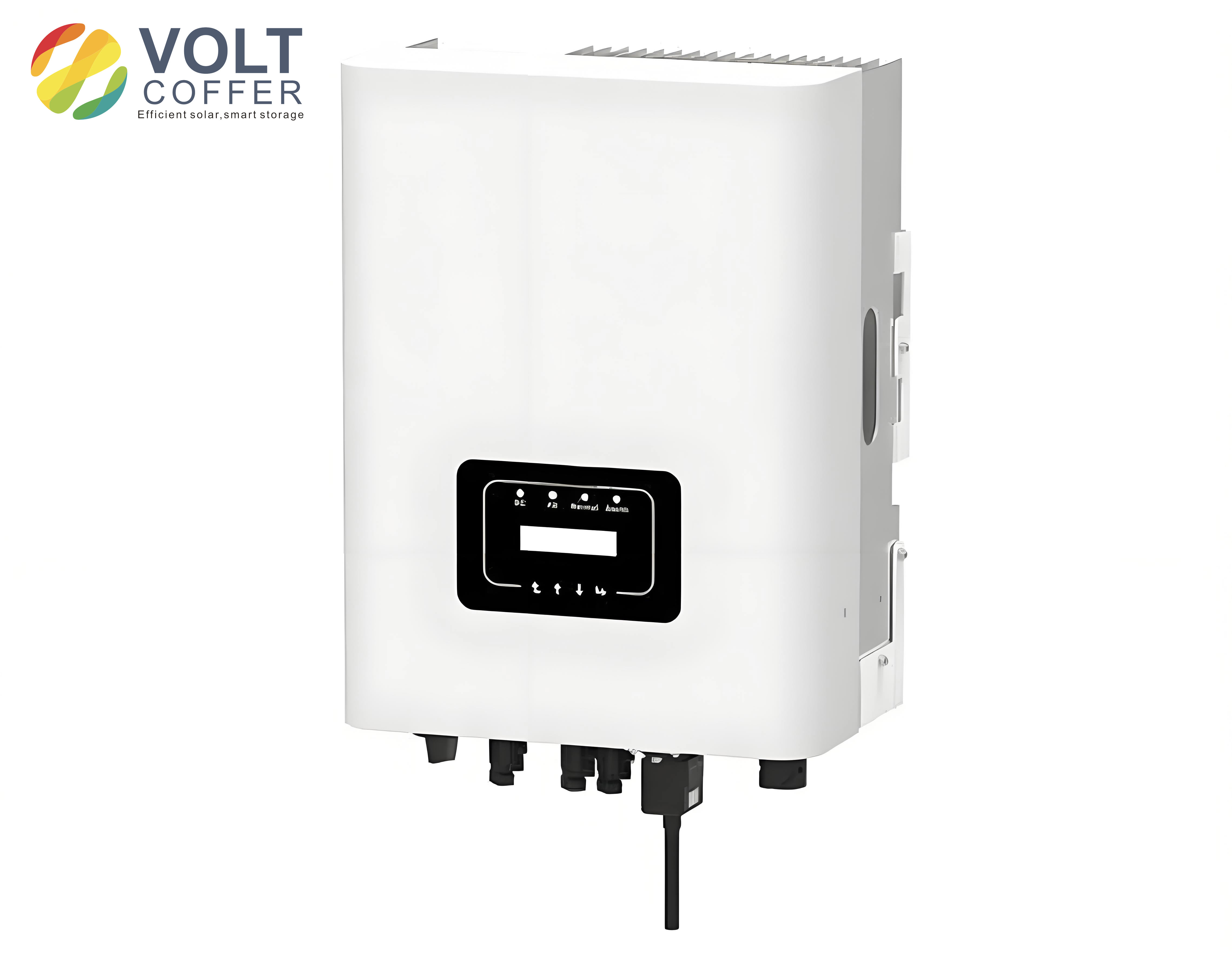
The solar inverter is a typical source of supraharmonics due to its high-frequency switching operation. In this work, I consider a three-phase L-type solar inverter, whose topology is shown in Figure 1 (conceptually). The inverter consists of six power switches S1–S6, an output filter inductance L1, a DC-link capacitor C, and the grid-side resistances R. The DC voltage Ed is supplied by the photovoltaic array, and the SPWM (sinusoidal pulse width modulation) strategy is employed to control the switches. The switching action generates voltage waveforms that contain a rich spectrum of harmonics, extending into the supraharmonic range.
The output phase voltage of a single-phase full-bridge bipolar SPWM inverter can be expressed as a Fourier series. For a given modulation wave $u_s(t) = U_s \sin(\omega_s t – \varphi)$ and a triangular carrier with frequency $f_c$, the frequency modulation ratio is defined as $N = f_c / f_s$, and the amplitude modulation ratio is $M = U_s / U_c$. The analytical expression of the output voltage contains components at the carrier frequency and its sidebands. In general, the harmonic frequencies are given by
$$ f_k = m f_c \pm n f_s = (mN \pm n) f_s $$
where $m$ and $n$ are integers. The corresponding amplitude is
$$ U_k = \frac{4 E_d}{m\pi} J_n\left(\frac{mM\pi}{2}\right) $$
where $J_n(\cdot)$ is the Bessel function of the first kind. These formulas indicate that supraharmonics mainly appear around the switching frequency and its multiples, and their amplitudes are directly related to the DC-side voltage.
2.2 Influence of Key Parameters
From the mathematical model, several important conclusions can be drawn. First, the frequency of supraharmonics is primarily determined by the switching frequency of the power devices. Second, the amplitude of supraharmonics depends on both the modulation ratio and the DC-side voltage. Third, the maximum power point tracking (MPPT) control strategy has a negligible influence on supraharmonic generation because the MPPT perturbation period (typically 30 ms) is much longer than the period of supraharmonics (6.7 μs to 500 μs). Therefore, I focus on the effects of switching frequency and DC-side voltage.
To verify the theoretical analysis, I built a simulation model of the solar inverter in MATLAB/Simulink. Three different switching frequencies were tested: 5 kHz, 12.5 kHz, and 20 kHz. The simulation results confirm that supraharmonic components are concentrated around the characteristic frequencies (switching frequency and its integer multiples). Table 1 summarizes the measured supraharmonic amplitudes near the characteristic frequencies for the case of 5 kHz switching frequency.
| Index | Around 5 kHz | Around 10 kHz | Around 15 kHz | |||
|---|---|---|---|---|---|---|
| Frequency (kHz) | Amplitude (%) | Frequency (kHz) | Amplitude (%) | Frequency (kHz) | Amplitude (%) | |
| 1 | 4.60 | 2.231 | 9.65 | 0.353 | 14.60 | 0.177 |
| 2 | 4.80 | 1.452 | 9.75 | 0.547 | 14.80 | 0.135 |
| 3 | 4.90 | 2.017 | 9.95 | 1.182 | 14.90 | 0.174 |
| 4 | 5.10 | 1.963 | 10.05 | 1.139 | 15.10 | 0.154 |
| 5 | 5.20 | 1.394 | 10.25 | 0.533 | 15.20 | 0.106 |
| 6 | 5.40 | 0.209 | 10.35 | 0.339 | 15.40 | 0.170 |
It is observed that the maximum supraharmonic amplitudes near the characteristic frequency exhibit a symmetric pattern. Specifically, when the characteristic frequency is an even multiple of the switching frequency, the sideband peaks appear at odd multiples of the fundamental frequency; conversely, when it is an odd multiple, the peaks appear at even multiples. This behavior is consistent with the theoretical prediction and confirms the close relationship between switching frequency and supraharmonic generation.
Furthermore, I investigated the effect of DC-side voltage on the supraharmonic amplitudes. The simulation results show that as the DC voltage increases, the supraharmonic content at the first sideband of the fundamental switching frequency decreases, while at the first sideband of the second harmonic of the switching frequency it increases. This is due to the fact that the modulation ratio changes inversely with the DC voltage, which in turn affects the harmonic amplitudes.
3. Compressed Sensing and Block Compressed Sensing
3.1 Fundamentals of Compressed Sensing
Compressed sensing (CS) is a signal acquisition paradigm that allows for the reconstruction of sparse signals from far fewer measurements than required by the Nyquist theorem. The CS measurement process can be modeled as
$$ \mathbf{y} = \mathbf{\Phi} \mathbf{x} = \mathbf{\Phi} \mathbf{\Psi} \mathbf{s} = \mathbf{A} \mathbf{s} $$
where $\mathbf{x}$ is the original signal of length $N$, $\mathbf{\Psi}$ is an $N \times N$ sparse basis matrix, $\mathbf{s}$ is the sparse coefficient vector, $\mathbf{\Phi}$ is an $M \times N$ measurement matrix (with $M \ll N$), $\mathbf{A} = \mathbf{\Phi}\mathbf{\Psi}$ is the sensing matrix, and $\mathbf{y}$ is the measured vector of length $M$. The signal $\mathbf{s}$ is said to be $K$-sparse if it contains at most $K$ non-zero elements.
The core requirements of CS are: (i) the signal must be sparse in some domain; (ii) the measurement matrix must satisfy the restricted isometry property (RIP) or, equivalently, be incoherent with the sparse basis; and (iii) a suitable recovery algorithm must be used to reconstruct the sparse coefficients from the measurements.
3.2 Sparsity of Supraharmonic Signals
Supraharmonic signals are not sparse in the time domain, but they can be sparsely represented in the frequency domain. Considering a typical current signal that contains multiple supraharmonic components, I model it as
$$ x(t) = \sum_{h} A_h e^{-\beta t} \cos(2\pi f_h t + \varphi_h) + n(t) $$
where $A_h$, $f_h$, and $\varphi_h$ are the amplitude, frequency, and phase of the $h$-th supraharmonic component, respectively, $\beta$ represents the damping factor, and $n(t)$ is noise. After discretization with sampling frequency $f_s$, the DFT of such a signal exhibits distinct peaks only at the frequencies corresponding to the supraharmonic components. Therefore, the superharmonic signal is compressible in the DFT basis. Figure 2 (not shown) illustrates the sparse representation of a simulated superharmonic signal using different bases, and the DFT basis provides the most concentrated representation.
3.3 Block Compressed Sensing for Supraharmonics
Traditional CS requires the use of a large measurement matrix, which consumes substantial memory and computational resources, especially for wideband superharmonic signals. To address this issue, I adopt the block compressed sensing (BCS) strategy. In BCS, the sparse signal is divided into several blocks, and each block is measured independently using the same measurement matrix. For a signal of length $N$ divided into $B$ blocks, each block has length $N/B$. The measurement matrix for each block is of size $(M/B) \times (N/B)$, and the overall measurement matrix is a block-diagonal matrix of the form
$$ \mathbf{\Phi} = \begin{bmatrix} \mathbf{\Phi}_B & \mathbf{0} & \cdots & \mathbf{0} \\ \mathbf{0} & \mathbf{\Phi}_B & \cdots & \mathbf{0} \\ \vdots & \vdots & \ddots & \vdots \\ \mathbf{0} & \mathbf{0} & \cdots & \mathbf{\Phi}_B \end{bmatrix} $$
This approach greatly reduces the memory footprint and allows for parallel processing of each block, thus enhancing computational efficiency.
To further minimize data volume, I propose a first-and-last-two-cycles sampling method based on the IEC 61000-4-30 framework. Instead of continuously sampling the entire 200 ms window, only the first and last 20 ms (one fundamental cycle) are selected for analysis. This scheme reduces the amount of sampled data to 20% of the total, while still preserving the characteristic features of superharmonics.
When applying BCS, I also need to handle the block edge effects. To mitigate these effects, I propose an overlapping block strategy where each block is extended by 1/16 of its length on both sides (except for the first and last blocks, which are extended by 1/8 on the outer side). This technique shifts the block boundaries away from the main signal content and improves reconstruction quality.
4. Improved Reconstruction Algorithm: ASCoSaMP
4.1 Compressive Sampling Matching Pursuit (CoSaMP)
CoSaMP is a well-known greedy algorithm for sparse signal recovery. It iteratively identifies the support set of the signal by selecting the largest correlation between the residual and the columns of the sensing matrix, and then solves a least-squares problem to estimate the signal coefficients. However, CoSaMP requires the sparsity level $K$ to be known in advance, which is often unavailable in practical applications. Moreover, its fixed number of iterations may lead to excessive computation.
4.2 Proposed ASCoSaMP Algorithm
To overcome these limitations, I develop an adaptive step-size sparsity-adaptive CoSaMP algorithm (ASCoSaMP). The key innovations include:
- Adaptive sparsity estimation: Instead of using a fixed sparsity, the algorithm starts with an initial sparsity $L$ and gradually increases $L$ during the iteration process until the true sparsity is approached.
- Variable step size: A step-length adjustment factor is introduced. When the residual is large, a larger step is used to quickly approach the true sparsity; when the residual becomes small, a smaller step is used to refine the estimate. The step size is updated as $L = L + \text{step} \cdot 0.5^{\zeta}$, where $\zeta$ is an adaptive parameter.
- Improved stopping criterion: In addition to the traditional residual-based stopping rule, I introduce a support set variation criterion. The iteration stops when the change in the support set between consecutive iterations is below a threshold, which speeds up convergence.
The detailed flow of the ASCoSaMP algorithm is summarized in Algorithm 1.
|
Input: sensing matrix $\mathbf{A}$, measurement vector $\mathbf{y}$, initial step size $S$, threshold $\eta_1, \eta_2$ Output: reconstructed sparse signal $\mathbf{s}$ 1: Initialize residual $\mathbf{r}_0 = \mathbf{y}$, support set $\Lambda_0 = \emptyset$, iteration counter $t=1$, sparsity estimate $L = S$. 2: while stopping criterion not met do 3: Compute correlation $\mathbf{u} = |\mathbf{A}^T \mathbf{r}_{t-1}|$. 4: Select indices of $2L$ largest entries of $\mathbf{u}$, form candidate set $J$. 5: Merge support: $\Lambda_t = \Lambda_{t-1} \cup J$. 6: Solve least squares: $\tilde{\mathbf{s}} = \arg\min_{\mathbf{s}} \|\mathbf{y} – \mathbf{A}_{\Lambda_t} \mathbf{s}\|$. 7: Keep only the largest $L$ entries of $\tilde{\mathbf{s}}$, and update the support set accordingly. 8: Compute new residual $\mathbf{r}_t = \mathbf{y} – \mathbf{A}_{\Lambda_t} \tilde{\mathbf{s}}$. 9: Update sparsity estimate using variable step size strategy. 10: $t \leftarrow t+1$. 11: end while 12: return $\mathbf{s}$ with values on the final support set. |
4.3 Performance Evaluation of ASCoSaMP
I evaluated the performance of the proposed ASCoSaMP algorithm against several classic reconstruction algorithms, including OMP, CoSaMP, SP, and SAMP. The test signal contained ten supraharmonic components with frequencies around 16 kHz, 32 kHz, 48 kHz, 64 kHz, and 80 kHz, representing the characteristic frequencies of a solar inverter with a 16 kHz switching frequency. The detailed signal parameters are listed in Table 2.
| Band | Frequency (kHz) | Amplitude (V) | Phase (°) |
|---|---|---|---|
| 1st harmonic | 15.85 | 58.48 | 206.9 |
| 16.15 | 57.96 | 85.1 | |
| 2nd harmonic | 31.85 | 18.84 | 74.2 |
| 32.15 | 18.04 | 38.7 | |
| 3rd harmonic | 47.85 | 4.92 | 76.3 |
| 48.15 | 4.80 | 190.9 | |
| 4th harmonic | 63.85 | 2.60 | 205.1 |
| 64.15 | 2.16 | 78.9 | |
| 5th harmonic | 79.85 | 3.78 | 79.3 |
| 80.15 | 3.40 | 90.7 |
Figure 3 shows the reconstruction success probability versus the compression ratio for the five algorithms. It is evident that ASCoSaMP achieves perfect reconstruction at a compression ratio of only 10%, whereas the other algorithms require at least 15% or more. This demonstrates that ASCoSaMP can significantly reduce the number of measurements needed.
Figure 4 illustrates the reconstruction success probability as a function of the signal sparsity. ASCoSaMP maintains a high success probability up to a sparsity level of 60, outperforming all other algorithms. This robustness is crucial for superharmonic signals, which may exhibit a relatively large number of spectral components.
I also compared the reconstruction accuracy in terms of mean square error (MSE) and signal-to-noise ratio (SNR) under a 40 dB noisy condition. The results are presented in Table 3.
| Algorithm | MSE | SNR (dB) | Computation time (s) |
|---|---|---|---|
| OMP | 3.8851 | 72.97 | — |
| CoSaMP | 3.8091 | 73.07 | — |
| SP | 3.7528 | 73.13 | — |
| SAMP | 0.5616 | 81.39 | 2.466 |
| ASCoSaMP | 0.5578 | 81.42 | 0.686 |
ASCoSaMP exhibits the lowest MSE and the highest SNR, while also being significantly faster than SAMP. This indicates that the proposed algorithm provides an excellent trade-off between accuracy and computational efficiency.
5. BCS-ASCoSaMP for Grid Supraharmonic Detection
5.1 Overall Framework
Combining the block compressed sensing strategy with the proposed ASCoSaMP reconstruction algorithm, I construct a complete detection method for grid supraharmonics. The processing flow is as follows:
- Preprocessing: Apply a Chebyshev type II bandpass filter to the input current or voltage signal to retain only the frequency components between 2 kHz and 150 kHz.
- First-and-last-two-cycles sampling: From a 200 ms time window, extract the first 20 ms and the last 20 ms as two analysis blocks.
- Sparse transformation: For each 20 ms block, apply the DFT basis to obtain the sparse coefficient vector.
- Block partitioning: Divide the sparse coefficient vector into 32 overlapping blocks according to the proposed strategy.
- Block-wise measurement: Multiply each block by a binary sparse random measurement matrix to obtain compressed measurements.
- Block-wise reconstruction: Reconstruct each block using the ASCoSaMP algorithm.
- Merging: Combine the reconstructed blocks to form the complete sparse spectrum.
- Parameter extraction: Identify the frequency and amplitude of each supraharmonic component from the spectrum.
- Result averaging: Repeat the process for both the first and the last 20 ms blocks, and average the estimated parameters to improve accuracy.
5.2 Simulation Results
5.2.1 Supraharmonics at Integer Multiples of 2 kHz
To validate the proposed method, I generated a test signal with eight supraharmonic components at frequencies that are integer multiples of 2 kHz, as listed in Table 4.
| Index | 1 | 2 | 3 | 4 | 5 | 6 | 7 | 8 |
|---|---|---|---|---|---|---|---|---|
| Frequency (kHz) | 4 | 12 | 16 | 30 | 50 | 80 | 120 | 150 |
| Amplitude (p.u.) | 0.8 | 0.7 | 0.6 | 0.5 | 0.45 | 0.4 | 0.3 | 0.2 |
The detection results obtained by the 32-DFT method, the CS-OMP method, and the proposed BCS-ASCoSaMP method are compared. All three methods are able to identify the frequencies and amplitudes correctly. However, the 32-DFT method has a lower frequency resolution, which may lead to spectral leakage when two components are closely spaced. In contrast, both CS-based methods provide much higher resolution.
To test the noise robustness, I added white Gaussian noise to the signal, resulting in SNRs of 30 dB, 40 dB, and 50 dB. For each noise level, I performed 100 independent trials and calculated the average estimated parameters. The maximum amplitude errors are summarized in Table 5. The BCS-ASCoSaMP method achieves the smallest errors, especially at low SNR.
| SNR | 32-DFT | CS-OMP | BCS-ASCoSaMP |
|---|---|---|---|
| 30 dB | 0.0045 | 0.0025 | 0.0012 |
| 40 dB | 0.0015 | 0.0007 | 0.0005 |
| 50 dB | 0.0008 | 0.0004 | 0.0003 |
5.2.2 Supraharmonics at Non-Integer Multiples of 2 kHz
In practice, supraharmonic frequencies are not necessarily aligned with 2 kHz intervals. Therefore, I used the signal parameters from Table 2, which are typical of a solar inverter with a 16 kHz switching frequency. Figure 5 compares the detection results of the 32-DFT method and the proposed BCS-ASCoSaMP method. The 32-DFT method fails to distinguish the closely spaced components and reports a single peak near each characteristic frequency, while BCS-ASCoSaMP resolves each component accurately.
Table 6 lists the estimated frequencies and amplitudes for BCS-ASCoSaMP, CS-OMP, and 32-DFT. It is clear that BCS-ASCoSaMP provides the most accurate estimates, with zero frequency error and maximum amplitude error below 0.7%, even at a 30 dB noise level.
| True frequency (kHz) | True amplitude (V) | 32-DFT f (kHz) | 32-DFT amp (V) | CS-OMP f (kHz) | CS-OMP amp (V) | BCS-ASCoSaMP f (kHz) | BCS-ASCoSaMP amp (V) |
|---|---|---|---|---|---|---|---|
| 15.85 | 58.48 | 16.0 | 77.77 | 15.8 | 55.01 | 15.85 | 58.48 |
| 16.15 | 57.96 | — | — | 16.2 | 16.94 | 16.15 | 57.96 |
| 31.85 | 18.84 | 32.0 | 35.44 | 31.8 | 21.02 | 31.85 | 18.84 |
| 32.15 | 18.04 | — | — | — | — | 32.15 | 18.04 |
| 47.85 | 4.92 | 48.0 | 2.99 | 47.8 | 3.07 | 47.85 | 4.92 |
| 48.15 | 4.80 | — | — | 48.2 | 2.95 | 48.15 | 4.80 |
| 63.85 | 2.60 | 64.0 | 3.08 | 63.8 | 1.27 | 63.85 | 2.60 |
| 64.15 | 2.16 | — | — | 64.2 | 0.96 | 64.15 | 2.16 |
| 79.85 | 3.78 | 80.0 | 2.42 | 79.8 | 2.92 | 79.85 | 3.78 |
| 80.15 | 3.40 | — | — | 80.2 | 1.45 | 80.15 | 3.40 |
5.2.3 Test with Solar Inverter Generated Supraharmonics
To further evaluate the practical applicability of the proposed method, I extracted supraharmonic components from the Simulink model of the solar inverter operating at a 5 kHz switching frequency. The six most significant components near the first, second, and third characteristic frequencies were selected, as shown in Table 7. The BCS-ASCoSaMP algorithm successfully recovered all the frequency and amplitude values. When 40 dB white noise was added, the maximum amplitude error remained below 1.1%, demonstrating the excellent noise immunity of the method.
| Index | Near 5 kHz | Frequency (kHz) | Amplitude (V) | Near 10 kHz | Frequency (kHz) | Amplitude (V) | Near 15 kHz | Frequency (kHz) | Amplitude (V) |
|---|---|---|---|---|---|---|---|---|---|
| 1 | 4.60 | 2.231 | 9.65 | 0.353 | 14.60 | 0.177 | |||
| 2 | 4.80 | 1.452 | 9.75 | 0.547 | 14.80 | 0.135 | |||
| 3 | 4.90 | 2.017 | 9.95 | 1.182 | 14.90 | 0.174 | |||
| 4 | 5.10 | 1.963 | 10.05 | 1.139 | 15.10 | 0.154 | |||
| 5 | 5.20 | 1.394 | 10.25 | 0.533 | 15.20 | 0.106 | |||
| 6 | 5.40 | 0.209 | 10.35 | 0.339 | 15.40 | 0.170 |
6. Experimental Validation with Real Supraharmonic Signals
6.1 Measurement Platform Description
To validate the proposed method in a real environment, I designed and implemented a supraharmonic measurement platform. The platform consists of a signal conditioning module, a high-speed ADC module (ADS8568), a DSP module (TMS320C6748), and a PC for data processing. The signal conditioning module uses a resistive voltage divider for voltage sensing and a manganese-copper shunt for current sensing, followed by a low-noise wideband operational amplifier (AD829) to match the ADC input range.
The ADC module employs the ADS8568, a 16-bit, 8-channel simultaneous sampling converter with a maximum sampling rate of 510 kHz, which is suitable for capturing signals up to 150 kHz. The DSP TMS320C6748 is a high-performance fixed/floating-point processor running at up to 456 MHz, providing sufficient computational power for real-time data handling. Communication between the DSP and the PC is achieved via a USB interface using the CH340G chip.
6.2 Experimental Results
I used an Agilent 33500 series signal generator to produce a test signal containing ten supraharmonic components with frequencies distributed between 10 kHz and 83 kHz. The actual signal was fed into the measurement platform, and the BCS-ASCoSaMP algorithm was applied. Table 8 shows the parameter estimation results from 100 repeated experiments.
| True frequency (kHz) | True amplitude (V) | Estimated frequency (kHz) | Estimated amplitude (V) | Frequency error | Amplitude error (%) |
|---|---|---|---|---|---|
| 10.2 | 6.0 | 10.2 | 6.003 | 0 | 0.047 |
| 19.1 | 5.7 | 19.1 | 5.702 | 0 | 0.030 |
| 31.85 | 4.8 | 31.85 | 4.799 | 0 | 0.019 |
| 32.15 | 4.5 | 32.15 | 4.501 | 0 | 0.030 |
| 41.3 | 4.0 | 41.3 | 4.002 | 0 | 0.012 |
| 53.85 | 3.5 | 53.85 | 3.501 | 0 | 0.024 |
| 60.0 | 3.3 | 60.0 | 3.298 | 0 | 0.058 |
| 72.15 | 2.5 | 72.15 | 2.502 | 0 | 0.074 |
| 80.2 | 2.2 | 80.2 | 2.199 | 0 | 0.052 |
| 83.1 | 1.7 | 83.1 | 1.697 | 0 | 0.150 |
The results demonstrate that the BCS-ASCoSaMP method achieves zero frequency error and a maximum amplitude error of only 0.15%. This confirms the practical feasibility and high accuracy of the proposed approach for real-world supraharmonic monitoring.
7. Conclusion and Future Work
In this thesis, I have conducted a comprehensive investigation into the generation mechanism and detection methods of supraharmonics in solar inverters. The main contributions and findings are summarized as follows:
- Generation mechanism: Through theoretical analysis and simulation, I verified that supraharmonics from a solar inverter are primarily caused by the high-frequency switching operation. The switching frequency directly determines the location of supraharmonic components, while the DC-side voltage affects their amplitudes through the modulation ratio. The MPPT control strategy has negligible influence on supraharmonic generation.
- Block compressed sensing detection: I established a mathematical model for supraharmonic signals and demonstrated their sparsity in the DFT domain. A block compressed sensing framework was developed, incorporating a first-and-last-two-cycles sampling method and an overlapping block strategy to reduce data volume and mitigate edge effects. The use of binary sparse random measurement matrices further enhances computational efficiency and memory savings.
- Improved reconstruction algorithm: I proposed the ASCoSaMP algorithm, which adaptively estimates the signal sparsity using a variable step-size approach and introduces an improved stopping criterion based on support set variation. This algorithm significantly outperforms existing methods such as OMP, CoSaMP, SP, and SAMP in terms of reconstruction accuracy and computational speed, particularly when the sparsity is unknown.
- Complete detection method: By integrating BCS with ASCoSaMP, I developed a complete supraharmonic detection method. Extensive simulations under various conditions (including integer and non-integer multiples of 2 kHz, noise contamination, and solar inverter generated signals) demonstrated that the method provides accurate frequency and amplitude estimation with strong noise robustness.
- Hardware validation: I constructed a supraharmonic measurement platform using the ADS8568 ADC and TMS320C6748 DSP. Real-world experiments confirmed that the proposed method achieves excellent performance, with maximum amplitude error below 0.15% for a ten-component test signal.
There are several areas that warrant further investigation. First, the current study focuses on a single solar inverter; future work could extend the analysis to multiple inverters with different switching frequencies operating in parallel, which would lead to more complex supraharmonic interactions. Second, the block size in the BCS framework is currently fixed; developing an adaptive block partitioning scheme based on the signal characteristics could further improve efficiency and accuracy. Third, the hardware implementation currently realizes the compressed sampling in the PC software; implementing random demodulation in hardware would enable true sub-Nyquist sampling and enhance the real-time capability of the system.
In summary, this research provides a solid theoretical foundation and practical guidance for the detection and analysis of supraharmonics in solar inverters, contributing to the safe and stable operation of modern power grids with high penetration of renewable energy sources.