
As the global energy transition accelerates, photovoltaic power generation has become a critical component of the renewable energy landscape. My research focuses on the anomaly detection of solar inverter output current using data mining techniques, addressing the challenge that inverter current is influenced by diverse factors including weather conditions, panel faults, and equipment operating states. The traditional anomaly detection methods exhibit high false detection rates and miss rates when applied to the complex, non-stationary current signals of solar inverters. Through systematic data preprocessing, clustering analysis, and deep learning model construction, I have developed effective anomaly detection approaches that significantly improve detection accuracy.
1. Introduction and Research Background
Solar energy, as one of the most abundant clean energy sources, has driven the rapid development of the photovoltaic power generation industry globally. According to data released by the National Energy Administration, China’s newly installed photovoltaic capacity reached 161 GW in the first three quarters of 2024, a year-on-year increase of 24.8%. By the end of September 2024, the total installed photovoltaic power generation capacity nationwide reached 770 GW, with photovoltaic power generation reaching 635.9 billion kWh in the first three quarters alone. Changqing Oilfield has actively responded to the global energy transition trend by introducing photovoltaic power generation projects, aiming to reduce dependence on fossil energy and promote the implementation of low-carbon emission reduction strategies.
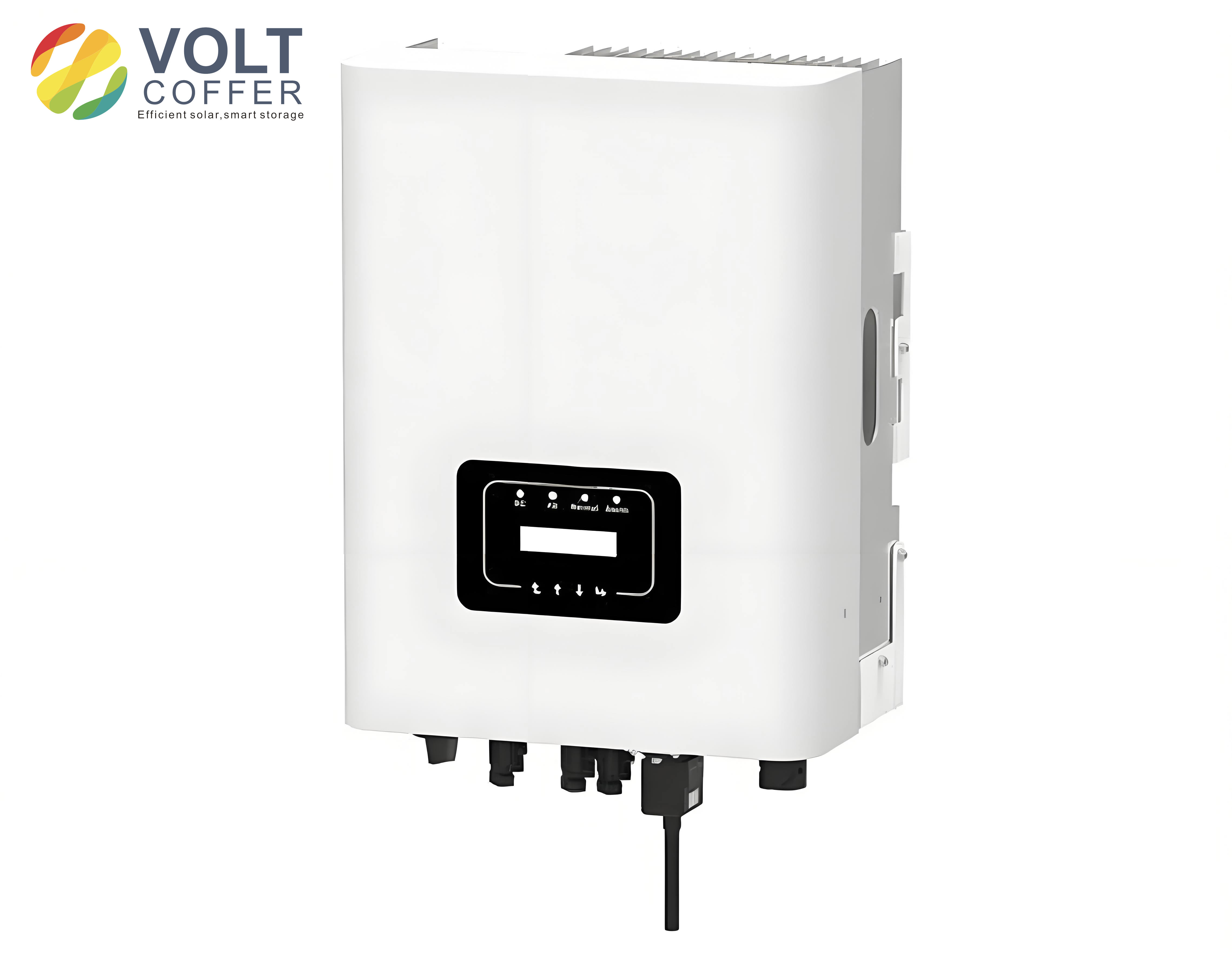
The solar inverter serves as the core equipment in photovoltaic power generation systems, responsible for converting DC power from solar panels into AC power compatible with the grid. The output current of the solar inverter directly reflects its operational status, and abnormal fluctuations in current can indicate various faults, including short circuits, open circuits, degradation of PV modules, or inverter internal failures. In long-term operation, solar inverters may encounter various faults that not only affect the normal operation of the photovoltaic system but may even cause electrical fires or electric shock safety hazards. Traditional manual inspection methods are labor-intensive, inefficient, and produce inconsistent quality results, failing to meet the modern photovoltaic industry’s demands for real-time monitoring, precision, and economic efficiency.
The distributed photovoltaic power generation systems are often located in remote and dispersed areas, making manual detection of solar inverter working status challenging. Recent advances in IoT technology and smart sensors have enabled the integration of data acquisition modules within solar inverters, facilitating real-time transmission and cloud storage of key operational parameters. This technological foundation has made data-driven operation and maintenance systems increasingly feasible, and my research leverages these capabilities to build a comprehensive anomaly detection framework for solar inverter current.
Anomaly detection identifies data points or sequences that significantly deviate from normal patterns. This field finds extensive applications across industrial equipment fault detection, credit card fraud detection, network security intrusion detection, and medical diagnostics. The common anomaly detection methods are generally classified into traditional approaches and deep learning-based approaches.
Traditional anomaly detection methods, also known as outlier detection, include statistical methods, distance-based methods, density-based methods, and clustering-based methods. Statistical methods such as z-score, 3-sigma principle, and boxplot establish a data distribution model and compute the probability that data objects conform to this model, classifying objects below a probability threshold as anomalies. While simple and computationally efficient, these methods rely heavily on the accuracy of the assumed statistical model and are suitable only for simple, low-dimensional datasets. The distance-based methods, including K-Nearest Neighbors (KNN) and Local Outlier Factor (LOF), use the distances between data points to quantify their similarity, but they suffer from high computational complexity in high-dimensional spaces. Density-based methods like DBSCAN and OPTICS analyze local density distributions, yet they are sensitive to parameter selection. Clustering-based methods such as K-means identify anomalies as data points not belonging to any cluster or significantly different from their cluster members.
The challenges faced by traditional anomaly detection methods in solar inverter current detection tasks are substantial. These include difficulty in selecting models that match the distribution of strongly fluctuating current data, high computational complexity in high-dimensional spaces, and incapability to adapt to the complex patterns of solar inverter currents, resulting in inaccurate detection outcomes and high false alarm rates.
In the context of big data, enhanced computational capabilities have powered the development of deep learning technologies, achieving remarkable progress in anomaly detection applications. Compared with traditional methods, deep learning approaches can process high-dimensional data and capture complex patterns within it, while also offering strong generalization capabilities and diverse data processing abilities that enable adaptation to various data distributions and anomaly types. Deep learning-based anomaly detection methods are commonly categorized into prediction-based and reconstruction-based approaches.
Prediction-based anomaly detection methods construct prediction models that use recent data windows to predict future points or subsequences, identifying points where the deviation between predicted and actual values exceeds a threshold. Common time series prediction algorithms include Long Short-Term Memory (LSTM), Convolutional Neural Networks (CNN), Temporal Convolutional Networks (TCN), and Transformer architectures. These algorithms have been successfully applied in solar inverter current prediction tasks. Wang Jing employed TCN with multi-scale feature fusion to capture and predict data trends, fitting the multivariate Gaussian distribution of prediction errors to evaluate anomaly scores. Ma Le designed an LSTM-DAGMM model and validated it with actual photovoltaic equipment data, demonstrating effective identification of anomalies in photovoltaic data. Reconstruction-based anomaly detection methods focus on reconstructing normal samples and calculating reconstruction errors between reconstructed values and original data, with samples whose reconstruction errors exceed a threshold identified as anomalies. Common reconstruction models include Autoencoder (AE), Variational Autoencoder (VAE), and Generative Adversarial Network (GAN). AE compresses input data into low-dimensional representations through an encoder and reconstructs the original data through a decoder, with its simplicity and efficiency making it widely applicable. Chen Lei proposed an LSTM-AE ensemble framework (LAEE) that increases the differentiation between reconstruction errors of normal and anomalous sequences, improving anomaly detection accuracy. Reconstruction-based methods achieve higher detection accuracy by fully reconstructing the system state from current time series data, offering advantages over prediction-based models.
Deep learning-based anomaly detection methods learn the internal features of normal data through neural network training, capturing complex temporal dependencies and maintaining detection performance stability through parameter adaptation. These methods consistently achieve higher accuracy and lower false positive rates compared with traditional anomaly detection approaches. For solar inverter current anomaly detection, the analysis of collected data requires sophisticated approaches because current patterns vary significantly across different weather conditions, making single-threshold methods inadequate. Consequently, in my research I introduced a clustering-based methodology that constructs distinct datasets for different weather conditions before applying anomaly detection models, significantly improving detection accuracy.
2. Data Processing and Analysis for Solar Inverter Current
2.1 Data Acquisition Framework
The data acquisition architecture for solar inverter monitoring follows a classic three-layer design: device layer (solar inverter), communication layer (4G gateway), and application layer (cloud platform). The acquisition process begins with connecting the solar inverter and 4G gateway via RS485 lines, collecting inverter data using the Modbus RTU protocol. The 4G gateway processes the data according to the Modbus RTU protocol and collection rules, then transmits the processed data to the cloud platform through the 4G wireless network. The cloud platform or host computer system receives the transmitted data through the wireless gateway’s IP address and MAC address, decodes it, and completes the data acquisition process. This architecture ensures reliable, real-time data transmission from solar inverters to the processing platform, forming the foundation for subsequent analysis.
The collected raw data attributes from solar inverter operations include A-phase current (nbq_ia), B-phase current (nbq_ib), C-phase current (nbq_ic), inverter efficiency (nbq_eff), A/B/C-phase voltages (nbq_ua, nbq_ub, nbq_uc), grid frequency (nbq_f), inverter internal temperature (nbq_t), voltage unbalance (dybp), AC active power (nbq_p), power factor (nbq_pf), over-temperature status (jngw), and short circuit status (nbdl). The sample data were collected at three-second intervals from a photovoltaic power station in Changqing Oilfield, providing a comprehensive view of solar inverter operational status. The raw data exhibit various quality issues including missing values, duplicates, and anomalies that require systematic preprocessing before analysis.
2.2 Data Preprocessing Methodologies
Data preprocessing constitutes a critical phase in data mining, ensuring the accuracy and effectiveness of subsequent analysis. My preprocessing workflow encompassed invalid attribute elimination, data resampling, missing value imputation, and anomaly data removal. The specific procedures are detailed below.
Invalid Attribute Elimination: The collected solar inverter data contained numerous attributes with high missing rates and values consistently equal to zero. These attributes, such as voltage unbalance, over-temperature status, and short circuit indicators, provide little value for current anomaly detection analysis. After eliminating these invalid attributes, the dataset retained 13 meaningful data items including date, nbq_ia, nbq_ib, nbq_ic, nbq_eff, nbq_ua, nbq_ub, nbq_uc, nbq_f, nbq_t, nbq_p, and nbq_pf.
Data Resampling: I applied downsampling to the time series data using the pandas resample function, converting the interval from every 3 seconds to every 10 minutes. Considering that the photovoltaic system operates between 5:30 and 20:30 daily, during which the solar inverter output current has practical effective values, I filtered data within this time range to reform the dataset. This adjustment significantly reduced data volume and redundancy while preserving the essential temporal patterns of solar inverter current.
Missing Value Imputation: The solar inverter operational data contained substantial missing values. I selected linear interpolation as the imputation method due to its computational simplicity and effectiveness for large datasets. The formula of linear interpolation is:
$$ \varphi_1(x) = \frac{x – x_0}{x_0 – x_1} y_0 + \frac{x – x_0}{x_1 – x_0} y_1 $$
After interpolation, I applied moving average smoothing to ensure stability of the imputed data. The moving average calculation is:
$$ SMA_t = \frac{x_1 + x_2 + \cdots + x_n}{n} $$
Anomaly Data Removal: Due to equipment failures, environmental factors, and data transmission issues, the collected solar inverter data contained anomalies. I replaced these anomalous values with missing values and used interpolation for imputation, thereby enhancing the data quality. This step prevented abnormal values from distorting the statistical properties of the dataset and degrading the performance of subsequently trained models.
2.3 Feature Selection using Principal Component Analysis
Feature selection identifies features that contribute most to the prediction model, reducing data dimensionality and removing redundant information. I employed Principal Component Analysis (PCA) as the primary feature selection technique, given the nonlinear relationships and high dimensionality inherent in solar inverter data. The PCA procedure involves several computational steps:
Given a sample matrix with n samples and p indicators, the standardized matrix is computed using the mean and standard deviation of each column:
$$ \bar{x}_j = \frac{1}{n}\sum_{i=1}^{n} x_{ij} $$
$$ S_j = \sqrt{\frac{\sum_{i=1}^{n}(x_{ij}-\bar{x}_j)^2}{n-1}} $$
$$ X_{ij} = \frac{x_{ij}-\bar{x}_j}{S_j} $$
The correlation coefficient matrix is then calculated as:
$$ r_{ij} = \frac{1}{n-1}\sum_{k=1}^{n} X_{ki} X_{kj} $$
Eigenvalues and eigenvectors are derived from the correlation coefficient matrix, followed by computing the contribution rate and cumulative contribution rate of principal components:
$$ b_i = \frac{\lambda_i}{\sum_{k=1}^{p}\lambda_k} $$
$$ \alpha_i = \frac{\sum_{k=1}^{i}\lambda_k}{\sum_{k=1}^{p}\lambda_k} $$
I performed PCA on the solar inverter data from March 30, 2023, excluding current and date attributes, retaining 8 attributes for analysis. The variance explained ratio plot indicated that when the number of principal components exceeded 5, the contribution rate began to stabilize, and the cumulative contribution rate reached over 90%. Therefore, I set the number of principal components to 5. The PCA results identified the five most contributing features as nbq_f (grid frequency), nbq_p (active power), nbq_t (inverter temperature), nbq_pf (power factor), and nbq_ub (B-phase voltage), with a cumulative contribution rate of 84%. Including the target feature nbq_ia (A-phase current), the final feature set comprised 6 attributes as summarized in Table 1.
| Feature | Meaning | Unit | Contribution Rate | Cumulative Contribution |
|---|---|---|---|---|
| nbq_f | Grid frequency | Hz | 0.249938 | 0.249938 |
| nbq_p | Active power | kW | 0.243829 | 0.493766 |
| nbq_t | Inverter temperature | ℃ | 0.157906 | 0.651672 |
| nbq_pf | Power factor | / | 0.114502 | 0.766174 |
| nbq_ub | B-phase voltage | V | 0.073489 | 0.839663 |
| nbq_ia | A-phase current | A | Target feature | Target feature |
2.4 Characteristic Analysis of Selected Features
Understanding the characteristics of each selected feature is essential for developing effective anomaly detection models for solar inverter current. The grid frequency serves as a critical indicator of power system stability. In China’s grid, the standard frequency is maintained at 50 Hz. During normal solar inverter operation, the grid frequency typically fluctuates within ±1 Hz around this nominal value, with deviations exceeding ±1 Hz signaling potential system instability. The normal operating frequency range for solar inverters in grid-connected mode is therefore between 49.5 Hz and 50.5 Hz.
Active power represents the actual effective power delivered to the grid by the photovoltaic system during grid-connected operation. The active power is closely correlated with voltage, current, and other electrical parameters; by measuring active power and considering known voltage and power factor, the output current of the solar inverter can be estimated. Under normal conditions, the active power should range between 80% and 100% of the rated power, with specific values varying according to system scale and environmental conditions. The inverter internal temperature typically ranges between 5℃ and 45℃ during normal operation of solar inverters. Exceeding this range may indicate an inverter fault. The power factor, expressed as cosφ, measures equipment efficiency, with values approaching 1 indicating higher efficiency. A power factor below 0.8 typically signals problems in the solar inverter or power system.
The B-phase voltage of the solar inverter normally fluctuates within a range of 220 to 250 V. The A-phase current is my target attribute for anomaly detection in this research. Through horizontal and vertical visualization analysis of the current data, I observed that the inverter current variation range is basically between 0 and 40 A. The current exhibits a fluctuating upward trend from morning to noon, reaching its maximum around midday, followed by a fluctuating downward trend from noon to evening. This characteristic reflects the close relationship between photovoltaic power generation and meteorological factors such as irradiance and temperature. However, actual weather conditions are variable and changeable, causing current values under different weather conditions to exhibit different fluctuation patterns.
According to observations of the collected data, the solar inverter current can be broadly categorized into three weather condition types: sunny, cloudy, and rainy days. Under sunny conditions, the inverter current changes smoothly, and the waveform resembles a Gaussian distribution. Under cloudy conditions, the current fluctuation is relatively large, with significant differences between maximum and minimum values. Under rainy conditions, due to the absence of sufficient solar irradiance, the fluctuation is relatively stable, with minimal differences between maximum and minimum values. For solar inverters, recognizing these distinct patterns is crucial for adapting anomaly detection strategies to different operational contexts.
2.5 Classification of Current Anomalies
Anomalies in the solar inverter current data can be broadly classified into three categories based on their characteristics: point anomalies, trend anomalies, and collective anomalies. Point anomalies, also known as global anomalies, occur when an individual data point deviates significantly from the majority of the dataset. In the solar inverter current sequence, most data points fall within the 0-40 A range; data points exceeding this range substantially constitute point anomalies. Trend anomalies refer to significant and unexpected changes in the long-term, relatively stable change pattern of the time series, such as rising, falling, or stable trends. Solar inverter current data typically exhibit periodic fluctuations; when data suddenly deviate from the original fluctuation trend, it may indicate solar inverter or photovoltaic system faults. Collective anomalies consist of multiple objects that may appear normal individually but collectively constitute an anomaly. In solar inverter current data, collective anomalies appear as sequences of abnormal points that may result from machine or system failures. The classification of anomaly types shown in Table 2 provides a systematic framework for evaluating detection model performance.
| Anomaly Type | Description | Example |
|---|---|---|
| Point anomaly | Individual data point significantly deviating from global majority | Current value above 40A |
| Trend anomaly | Significant unexpected change in long-term trend pattern | Sudden deviation from periodic fluctuation |
| Collective anomaly | Group of points appearing normal individually but anomalous together | Sequence of abrupt current changes |
2.6 Data Clustering Using DTW-K-means
The solar inverter current data exhibit different characteristics under different weather conditions, influenced by meteorological factors. Data under the same weather condition exhibit similar patterns, suggesting that anomaly detection algorithms applied to current data under specific weather conditions can effectively improve detection accuracy. Therefore, I proposed clustering the solar inverter current data to construct datasets under different weather conditions.
The K-means algorithm is simple and efficient, with the number of clusters K set according to common weather types. However, K-means relies on Euclidean distance, which cannot provide accurate similarity measures when handling nonlinearly deformed time series data. To address this limitation, I employed the Dynamic Time Warping (DTW) algorithm, which measures the similarity between time series by finding the optimal warping path with minimum cumulative distance through dynamic programming. DTW distance is more effective than Euclidean distance for solar inverter data characterized by significant fluctuations and periodic changes, making DTW-K-means better suited for this clustering task.
The DTW distance calculation process includes constructing the distance matrix between two sequences Q and S:
$$ W = \begin{bmatrix} d(q_1,s_1) & d(q_1,s_2) & \cdots & d(q_1,s_Y) \\ d(q_2,s_1) & d(q_2,s_2) & \cdots & d(q_2,s_Y) \\ \vdots & \vdots & \vdots & \vdots \\ d(q_X,s_1) & d(q_X,s_2) & \cdots & d(q_X,s_Y) \end{bmatrix} $$
The DTW distance between two sequences is defined as:
$$ DTW(Q,S) = \min \sum_{r=1}^{k} d(p_r) $$
The dynamic programming formulation for DTW distance is:
$$ DTW(Q,S) = D(n,m) = w_{nm} + \min\{D(n-1,m), D(n,m-1), D(n-1,m-1)\} $$
where D(0,0)=0, D(X,0)=D(0,Y)=+∞.
The clustering process used statistical features of solar inverter current including mean, maximum, minimum, standard deviation, and variance. The K-means algorithm with k=3 produced clusters representing sunny, cloudy, and rainy day datasets. However, as shown in the experimental results, the classification boundaries between adjacent weather categories were not clear with standard K-means. The DTW-K-means algorithm achieved better separation between different current categories, effectively distinguishing solar inverter currents under various weather conditions, thereby creating more homogeneous datasets for subsequent anomaly detection and improving overall detection accuracy.
The clustering process using DTW-K-means algorithm is described in Table 3, providing the detailed steps for constructing weather-condition-specific solar inverter datasets.
| Step | Operation | Description |
|---|---|---|
| 1 | Input | Solar inverter current dataset with statistical features (mean, max, min, std, variance) |
| 2 | Initialize | Select k=3 initial cluster centroids |
| 3 | Assign | Calculate DTW distance between each data point and cluster centroids; assign each point to the nearest cluster |
| 4 | Update | Recalculate cluster centroids as the average of all data points in each cluster |
| 5 | Iterate | Repeat steps 3-4 until centroids no longer change significantly or maximum iteration is reached |
| 6 | Output | Three clusters representing sunny, cloudy, and rainy day solar inverter current datasets |
3. Anomaly Detection Models for Solar Inverter Current
Having established the clustered datasets, I proceeded to construct two distinct anomaly detection models: VMD-BiGRU and FFT-AE. These models represent different paradigms of anomaly detection, prediction-based and reconstruction-based respectively, and their comparison provides valuable insights into the most effective approach for solar inverter current anomaly detection.
3.1 VMD-BiGRU Anomaly Detection Model
Variational Mode Decomposition (VMD) is an adaptive, completely non-recursive modal variation and signal processing method. Its primary objective is to find an optimal modulation function that decomposes input signals into multiple Intrinsic Mode Functions (IMFs), each with specific frequencies and bandwidths that effectively represent the intrinsic structure and characteristics of the signal. Solar inverter current data are characterized by strong fluctuations and instability, and VMD effectively decomposes these current signals to extract meaningful patterns for enhanced feature representation.
The VMD algorithm generates k modal components with limited bandwidth and center frequency through an optimized variational approach. The constrained variational expression is:
$$ \min \left\{ \sum_{k=1}^{K} \left\| \partial_t \left[ \left(\delta(t) + \frac{j}{\pi t}\right) \times u_k \right] \exp(-j\omega t) \right\|_2^2 \right\} $$
subject to the constraint:
$$ \sum_{k=1}^{K} u_k = f(t) $$
where ∂t denotes the partial derivative, k denotes total component number, j denotes the imaginary unit, δ(t) is the Dirac distribution function, u_k represents the modal function set, ω_t represents the center frequency set, and f(t) represents the original signal.
Through introducing the penalty parameter α and the Lagrange multiplier operator λ, the constrained variational problem is transformed into an unconstrained variational problem. The augmented Lagrange expression is given by:
$$ L(\{u_k\},\{\omega_k\},\lambda) = \alpha \sum_k \left\| \partial_t \left[ \left(\delta(t) + \frac{j}{\pi t}\right) * u_k(t) \right] e^{-j\omega_l t} \right\|_2^2 + \left\| f(t) – \sum_k u_k(t) \right\|_2^2 + \langle \lambda(t), f(t) – \sum_k u_k(t) \rangle $$
The intrinsic mode functions and center frequencies are iteratively updated until convergence. In my implementation, I set the VMD decomposition modal number to 3 for solar inverter current data. The decomposition results for sunny weather conditions revealed that IMF1 reflects periodic patterns on a daily basis, IMF2 exhibits slightly larger amplitude fluctuations influenced by strongly correlated features, and IMF3 shows minimal variation reflecting weak correlation influences.
Gated Recurrent Unit (GRU) is a recurrent neural network architecture proposed for handling sequence data, addressing the gradient vanishing and explosion problems of traditional RNNs in long sequences. Compared with LSTM, GRU has only two gates: an update gate and a reset gate. The update gate combines the input gate and forget gate of LSTM, controlling the proportion of previous hidden state information retained in the current state and the degree of new information introduction. The reset gate controls the proportion of past information forgotten. The GRU network structure offers simplified architecture and faster training speed, achieving similar performance to LSTM in many tasks. The GRU computational process is governed by the following equations:
$$ z_t = \sigma(W_z \cdot [h_{t-1}, x_t]) $$
$$ r_t = \sigma(W_r \cdot [h_{t-1}, x_t]) $$
$$ \hat{h}_t = \tanh(W \cdot [r_t \odot h_{t-1}, x_t]) $$
$$ h_t = (1 – z_t) \odot h_{t-1} + z_t \odot \hat{h}_t $$
where σ denotes the sigmoid activation function, ⊙ denotes element-wise multiplication, W_z and W_r denote the weight matrices of the update gate and reset gate, h_{t-1} is the previous hidden state, and x_t is the current input vector.
GRU networks, while overcoming gradient issues, can only describe dependencies in a single direction, processing sequence data from front to back. This limitation prevents the model from fully exploring the inherent features and bidirectional dependencies of sequence data. Bidirectional Gated Recurrent Unit (BiGRU) overcomes this limitation by using two independent GRU units: one processes data forward in the time sequence, and the other processes data backward. For solar inverter time series, BiGRU captures both forward and backward information simultaneously, thereby improving feature extraction and prediction accuracy. The BiGRU model computational process:
$$ \overrightarrow{h}_t = GRU(x_t, \overrightarrow{h}_{t-1}) $$
$$ \overleftarrow{h}_t = GRU(x_t, \overleftarrow{h}_{t-1}) $$
$$ h_t = \omega_t \overrightarrow{h}_t + v_t \overleftarrow{h}_t + b_t $$
where ω_t and v_t are the weights of the forward and backward hidden states at time step t, and b_t is the bias term.
The threshold determination for anomaly detection using residuals between predicted and actual values is critical for solar inverter current anomaly detection. I evaluated two statistical methods: z-score and boxplot. The z-score method measures the standard deviation distance between data points and the mean:
$$ z\text{-}score = \frac{x – \mu}{\sigma} $$
In a standard normal distribution, approximately 99.7% of data points lie within 3 standard deviations of the mean. Data points with z-score absolute values exceeding 3 are likely anomalies. The boxplot method uses quartiles to identify anomalies:
$$ IQR = Q_3 – Q_1 $$
$$ L = Q_1 – k \times IQR $$
$$ W = Q_3 + k \times IQR $$
where Q_1 and Q_3 are the 25th and 75th percentiles, respectively, and k is typically 1.5.
The VMD-BiGRU anomaly detection model for solar inverter current operates through a structured workflow. The first step involves data preprocessing and clustering, where raw inverter data undergo cleaning and feature selection, and the DTW-K-means algorithm clusters data into sunny, cloudy, and rainy day datasets. The second step performs VMD decomposition on the current data of each weather dataset, generating IMF1, IMF2, …, IMFn modes that are added to the clustered dataset as new features to enhance data quality. The third step inputs the augmented new dataset into the BiGRU network model for training, using the trained model to predict current values. The fourth step computes residuals between predicted and actual current values to assess the anomaly extent. The fifth step uses z-score anomaly detection on residuals, setting thresholds to mark current data exceeding the threshold as anomalies. The complete workflow for the VMD-BiGRU solar inverter current anomaly detection model is presented in the system architecture, encompassing data preprocessing through anomaly classification.
3.2 FFT-AE Anomaly Detection Model
Fast Fourier Transform (FFT) serves as the mathematical foundation for converting time-domain signals to frequency-domain signals. FFT decomposes a complex signal into a linear combination of multiple sine and cosine waves of different frequencies. For solar inverter current analysis, I introduced FFT to convert time-domain current signals into frequency-domain signals, clearly identifying the amplitude and frequency of harmonics. The Discrete Fourier Transform is given by:
$$ X[k] = \sum_{n=0}^{N-1} x[n]e^{-j\frac{2\pi}{N}kn} $$
where N is the total number of signal samples, X[k] is the k-th frequency component in the frequency domain, and x[n] is the n-th sample in the time domain. The DFT complexity is O(N²). FFT exploits the odd-even, real-imaginary properties of DFT to achieve a complexity of O(N log N):
$$ f_{even}[n] = x[2n], \quad f_{odd}[n] = x[2n+1] $$
$$ \omega_N^k = e^{-2\pi i\frac{k}{N}} $$
$$ X[k + \frac{N}{2}] = F_{even}[k] + \omega_N^k F_{odd}[k], \quad k = 0, 1, \ldots, \frac{N}{2} – 1 $$
Autoencoder (AE) is trained through unsupervised learning to learn effective data representations. The AE structure consists of an encoder and a decoder. The encoder compresses input data into a low-dimensional latent variable:
$$ z = f(w^{(1)}x + b^{(1)}) $$
The decoder reconstructs the original data from the latent variable:
$$ x’ = f(w^{(2)}z + b^{(2)}) $$
The reconstruction error between reconstructed and original data is measured using Mean Squared Error as the loss function:
$$ MSE = \frac{1}{n}\sum_{i=1}^{n}(x_i – x_i’)^2 $$
Since autoencoders learn normal patterns from training data, input data significantly different from these normal patterns result in substantially increased reconstruction errors, enabling the identification of anomalous data points. This characteristic makes AE an important anomaly detection tool.
The FFT-AE model for solar inverter current anomaly detection operates through a comprehensive workflow. The first step performs current data preprocessing and clustering, including data resampling, alignment, missing value imputation, and DTW-K-means clustering. The second step uses FFT to convert solar inverter current time-domain signals into frequency-domain signals, identifying larger amplitude frequency components while removing noise and secondary information to reduce data redundancy. The third step processes the transformed frequency-domain data through the autoencoder, where the encoder compresses high-dimensional input data into low-dimensional latent space, and the decoder reconstructs features from the learned low-dimensional representation. The fourth step performs Inverse Fast Fourier Transform (IFFT) on the reconstructed frequency-domain features to convert back to time-domain signals, obtaining reconstructed original current data. The fifth step calculates reconstruction errors between original and reconstructed current data and uses z-score method for anomaly identification, marking data points whose residual values exceed the threshold as anomalous current values. This approach leverages the complete current time series to reconstruct the system state, achieving high detection accuracy.
3.3 Experimental Results and Model Evaluation
The experimental environment used for model construction and evaluation comprises a Windows 11 operating system, 12th Gen Intel Core i5-12500H CPU, NVIDlA GeForce RTX 3050 Laptop GPU, PyCharm 2022.2.3 IDE, TensorFlow 2.15.0 framework, Python 3.9.13 programming language, Scikit-learn 1.0.2, NumPy 1.21.5, and Pandas 1.4.4 libraries.
I used actual operational data from Changqing Oilfield photovoltaic power station, covering the period from March 22, 2023 to September 30, 2023. After resampling, the dataset contained 17,509 records. Using the solar inverter current as the target attribute for clustering, the dataset was divided into three weather categories. The sunny day dataset included 11,640 records, with 8,148 for training and 3,492 for testing. The cloudy day dataset contained 4,005 records, with 2,800 for training and 1,205 for testing. The rainy day dataset contained 1,864 records, with 1,300 for training and 564 for testing. Table 4 summarizes the dataset partitioning strategy.
| Weather Condition | Total Records | Training Set | Test Set |
|---|---|---|---|
| Sunny | 11,640 | 8,148 | 3,492 |
| Cloudy | 4,005 | 2,800 | 1,205 |
| Rainy | 1,864 | 1,300 | 564 |
| Total | 17,509 | 12,248 | 5,261 |
The VMD-BiGRU model parameters were optimized through multiple experimental iterations. The final configuration includes 3 VMD decomposition modes, a time step of 90 minutes, learning rate of 0.001, batch size of 32, 100 training epochs, Adam optimizer, MSE loss function, and residual threshold multiplier of 2.5. The parameter details are presented in Table 5.
| Parameter | Value |
|---|---|
| VMD decomposition modes | 3 |
| Time step | 90 minutes |
| Learning rate | 0.001 |
| batch_size | 32 |
| Epoch | 100 |
| Optimizer | Adam |
| Loss function | MSE |
| Residual threshold multiplier | 2.5 |
For the FFT-AE model, the parameter settings include a learning rate of 0.001, 100 epochs, Adam optimizer, MSE loss function, residual threshold multiplier of 3, 200 retained FFT frequencies, and 200 autoencoder input dimensions. The residual threshold used for FFT-AE identifies data points as anomalous when the residual exceeds three times the local mean. Table 6 summarizes these parameters.
| Parameter | Value |
|---|---|
| Learning rate | 0.001 |
| Epoch | 100 |
| Optimizer | Adam |
| Loss function | MSE |
| Residual threshold multiplier | 3 |
| FFT retained frequency count | 200 |
| Autoencoder input dimension | 200 |
To verify the effectiveness of the clustering method in anomaly detection tasks, I first applied traditional statistical anomaly detection methods including fixed threshold, boxplot, and z-score on both pre-clustering and post-clustering datasets. The fixed thresholds for solar inverter current under different conditions were set based on the operational ranges identified through data analysis, as shown in Table 7. For the pre-clustering dataset, the lower threshold was 0A and the upper threshold was 40A. For the post-clustering datasets, the sunny day current thresholds were 0-40A, cloudy day current thresholds were 0-30A, and rainy day current thresholds were 0-20A.
| Category | Indicator | Threshold |
|---|---|---|
| Pre-clustering | Current | Lower 0A, Upper 40A |
| Post-clustering Sunny | Current | Lower 0A, Upper 40A |
| Post-clustering Cloudy | Current | Lower 0A, Upper 30A |
| Post-clustering Rainy | Current | Lower 0A, Upper 20A |
The anomaly detection results before and after clustering reveal significant performance differences. Before clustering, the three methods detected only 38, 48, and 73 anomalies respectively out of 347 actual anomalies, indicating poor detection sensitivity and high miss rates. After clustering, the fixed threshold method detected 56 anomalies, boxplot detected 182 anomalies, and z-score detected 95 anomalies. While the total detection counts improved after clustering, the traditional methods still exhibited substantial miss rates and false positive rates. This finding motivated the application of deep learning anomaly detection models on the clustered datasets.
After establishing the limitations of traditional methods, I applied VMD-BiGRU and FFT-AE models on the clustered datasets. Table 8 presents the anomaly detection results for both models across different weather conditions.
| Detection Indicator | Actual Anomalies | VMD-BiGRU | FFT-AE |
|---|---|---|---|
| Sunny current | 53 | 57 | 51 |
| Cloudy current | 29 | 33 | 30 |
| Rainy current | 32 | 27 | 31 |
| Total after clustering | 114 | 117 | 112 |
The visualization of anomaly detection results for both models reveals important insights. In the plotted results, blue lines represent actual data, orange lines represent predicted or reconstructed data, green lines represent residual data from subtracting reconstructed or predicted values from actual values, red dashed lines represent the threshold set for residuals, and red points indicate detected anomalies. The visual analysis demonstrates that both models effectively identify solar inverter current anomalies, with the residual distribution remaining within expected bounds for normal data and exceeding thresholds at anomaly locations.
For quantitative model evaluation, I used the confusion matrix framework. The detection results are classified into four categories: True Positive (TP), False Negative (FN), False Positive (FP), and True Negative (TN). The confusion matrix structure is presented in Table 9.
| Actual Result | Anomaly Detected | Normal Detected |
|---|---|---|
| Anomaly | TP | FN |
| Normal | FP | TN |
From the confusion matrix, I computed precision, recall, accuracy, and F1 score as performance evaluation metrics:
$$ Precision = \frac{TP}{TP + FP} $$
$$ Recall = \frac{TP}{TP + FN} $$
$$ Accuracy = \frac{TP + TN}{TP + TN + FP + FN} $$
$$ F1Score = \frac{2 \times Precision \times Recall}{Precision + Recall} $$
The model evaluation results for each weather condition are shown in Tables 10 through 12, providing a comprehensive assessment of both anomaly detection models for solar inverter current under different operational contexts.
| Model | F1Score | Accuracy | Recall |
|---|---|---|---|
| VMD-BiGRU | 93.09 | 93.50 | 92.81 |
| FFT-AE | 94.30 | 96.10 | 96.11 |
| Model | F1Score | Accuracy | Recall |
|---|---|---|---|
| VMD-BiGRU | 90.53 | 91.68 | 91.10 |
| FFT-AE | 95.10 | 96.57 | 95.73 |
| Model | F1Score | Accuracy | Recall |
|---|---|---|---|
| VMD-BiGRU | 93.51 | 95.73 | 94.42 |
| FFT-AE | 97.50 | 98.60 | 97.25 |
The comprehensive evaluation results averaged across all weather conditions are presented in Table 13, providing an overall comparison of both models’ performance in solar inverter current anomaly detection.
| Model | F1Score | Accuracy | Recall |
|---|---|---|---|
| VMD-BiGRU | 92.37 | 93.64 | 92.78 |
| FFT-AE | 95.63 | 97.09 | 96.36 |
From the evaluation results, several important observations emerge regarding solar inverter current anomaly detection. In sunny and cloudy weather conditions, FFT-AE performed slightly better than VMD-BiGRU. This performance difference stems from the distinct algorithmic mechanisms of the two models. The VMD-BiGRU model predicts current values based on historical time series data, which introduces inherent lag in learning continuously changing current characteristics, causing prediction error accumulation and affecting anomaly detection accuracy. In contrast, the FFT-AE model reconstructs current data based on frequency-domain features of the current moment, bypassing time-series dependency delays and effectively improving reconstruction accuracy.
Both models achieved optimal detection performance on rainy day datasets, which is attributable to the characteristics of rainy day current data. Under rainy conditions, the current exhibits relatively small fluctuations and stable variations, effectively suppressing time-series prediction errors in VMD-BiGRU and significantly reducing frequency-domain reconstruction errors in FFT-AE. This finding confirms that data clustering by weather conditions enhances the overall performance of anomaly detection models for solar inverter current.
From the comprehensive evaluation, both models achieved evaluation indicators above 90%, indicating effective anomaly detection performance that meets the requirements of anomaly detection tasks. FFT-AE’s comprehensive indicators were slightly better than VMD-BiGRU, demonstrating its superior performance in solar inverter current anomaly detection tasks. The reconstruction-based approach of FFT-AE, leveraging complete current time series data to reconstruct system state, provides higher detection accuracy than the prediction-based approach.
4. System Design and Implementation
4.1 System Requirements Analysis
Based on the practical requirements identified through investigation of small photovoltaic power station operations, I designed the solar inverter current anomaly detection system with four primary functional modules. The system management module manages system users and data through five sub-modules: user management, role management, department management, menu management, and log management. Access control is implemented based on user roles, with system administrators having all management permissions and regular users having query-only permissions. The data management module manages solar inverter information and collected data, with key indicators displayed through curve charts for intuitive observation of inverter output data. The prediction and anomaly detection module performs current prediction and anomaly detection on collected solar inverter current indicators, enabling staff to take preventive measures based on analysis results, reducing inverter downtime and improving system reliability and generation efficiency. The operation and maintenance record management module consists of alarm records and maintenance records. Alarm records document anomalous solar inverter operating states for prompt response and problem resolution, while maintenance records document detailed information for each maintenance session, providing important data support for subsequent equipment maintenance and fault analysis.
4.2 Technical Architecture Design
The system uses Java and Python as the programming languages, based on Springboot and Vue frameworks, implementing a front-end and back-end separated architecture. The technical architecture is organized into three layers according to data interaction flow: data layer, service layer, and view layer. The data layer stores and accesses data using MySQL as the primary database, with Redis caching hot data to ensure fast system response times. The service layer implements business logic and rules through four sub-layers: data application layer, foundation layer, core framework layer, and control layer, separating business logic from data access logic for modularity and maintainability. The data application layer uses MyBatis for object-relational mapping, Alibaba Druid for database connection pool management, Hibernate Validation for parameter validation, and PageHelper for pagination. The foundation layer provides JDK, Maven, and Logback for logging. The core framework layer uses Spring Framework including Springboot and Spring Security. The control layer uses SpringMVC architecture.
The view layer uses Vue.js framework with Element UI for user interface components and Axios for HTTP communication, providing a clean and user-friendly interaction interface while ensuring reliable communication with the backend services.
4.3 Database Design
The database design process followed three stages: conceptual model design, logical structure design, and database table design. Through entity identification, the system incorporates two main entity categories: solar inverter system management entities (user information, role information, menu information, department information, log information, and maintenance records) and solar inverter data management entities (inverter information, collection information, prediction results, anomaly detection results, and alarm information). The logical structure design converted the E-R diagrams into database schema including fourteen main tables: user table, role table, menu table, department table, user-role table, role-menu table, login log table, operation log table, solar inverter information table, inverter collection data table, alarm information table, repair information table, prediction result table, and anomaly detection result table.
The solar inverter collection information table structure is detailed in Table 14, storing critical operational data from solar inverters including voltage, current, power, temperature, and power factor measurements.
| Field | Type | Length | Constraint | Description |
|---|---|---|---|---|
| cj_id | bigint | 20 | Primary key, auto-increment | ID |
| date | datetime | – | Not null | Collection time |
| inverter_id | varchar | 255 | Not null | Solar inverter ID |
| nbq_ub | varchar | 50 | Not null | B-phase voltage |
| nbq_ua | varchar | 50 | Not null | A-phase voltage |
| nbq_uc | varchar | 50 | Not null | C-phase voltage |
| nbq_ia | varchar | 50 | Not null | A-phase current |
| nbq_ib | varchar | 50 | Not null | B-phase current |
| nbq_ic | varchar | 50 | Not null | C-phase current |
| nbq_p | varchar | 50 | Not null | Active power |
| nbq_t | varchar | 50 | Not null | Temperature |
| nbq_eff | varchar | 255 | Not null | Power factor |
| day_generation | varchar | 255 | Not null | Daily generation |
| total_generation | varchar | 255 | Not null | Total generation |
| status | tinyint | 1 | Not null | Status |
| beizhu | varchar | 255 | Not null | Remarks |
4.4 System Function Implementation
The implemented system provides comprehensive functionality for solar inverter current anomaly detection. The system login interface allows users to input usernames, passwords, and digital verification codes for secure access. The data monitoring module displays the current operating status of the photovoltaic system through real-time monitoring data, system overview, power data, manufacturer statistics, and alarm records, presented through line charts, pie charts, and tables. Users can quickly understand the working status of the photovoltaic system and solar inverters, ensuring high-efficiency and stable operation.
The system management module includes user management, role management, menu management, department management, and log management sub-modules. User management enables administrators to create, edit, and delete user accounts. Role management defines different roles and assigns corresponding permissions to each role, with users obtaining operation permissions through their roles. Menu management defines the system menu structure and dynamically presents menu items based on user roles and permissions. Department management provides a hierarchical organizational structure. Log management records key system operational information, including login logs and operation logs.
The data management module includes solar inverter information, collection data, and voltage-current visualization sub-modules. The solar inverter information sub-module records and maintains basic inverter information including model, manufacturer, installation location, and operating status, supporting batch import and export. The collection data sub-module focuses on real-time and historical data collection, storage, and management, collecting operational data including input/output voltages, currents, active power, and conversion efficiency. The voltage-current visualization sub-module displays solar inverter current and voltage operating data through intuitive line charts, enabling users to quickly understand equipment output status and identify data trends, patterns, and anomalies.
The prediction and anomaly detection module includes data prediction and anomaly detection core sub-modules. Current prediction analyzes historical and real-time data using prediction algorithms to forecast future current trends. The current anomaly detection sub-module quickly identifies data points or behaviors that do not conform to normal patterns, helping the system pre-identify potential anomalous situations, take preventive measures, reduce the occurrence of abnormal events, and allow operation and maintenance personnel to promptly handle anomalies, ensuring system security and reliability.
The operation and maintenance record management module includes alarm records and maintenance records sub-modules. The alarm records sub-module collects and stores various alarm information generated during system operation, with detailed records of alarm time, level, type, and description, allowing operation personnel to quickly locate problem sources and take timely measures. The maintenance records sub-module records equipment maintenance history, covering maintenance time, content, personnel, and results, enabling operation teams to comprehensively understand equipment health status, reasonably arrange preventive maintenance plans, and extend equipment service life.
4.5 System Testing
System testing is a critical phase in the software development process, verifying that the system meets functional, performance, and security requirements in a simulated real environment. I conducted comprehensive functional testing on each module of the solar inverter current anomaly detection system. Table 15 presents the login function test case, validating system access control.
| Step | Operation Description | Expected Result | Actual Result |
|---|---|---|---|
| 1 | Input incorrect username | Indicate user name or password error | Consistent with expectation |
| 2 | Correct username with wrong password | Indicate user name or password error | Consistent with expectation |
| 3 | Incorrect verification code | Indicate verification code error | Consistent with expectation |
| 4 | Any field left empty | Indicate please fill in complete information | Consistent with expectation |
| 5 | Correct username, password, and code | Login successful | Consistent with expectation |
The user management module test cases validated user creation, editing, deletion, and query operations. Data management module testing confirmed the correct display and management of solar inverter information, accurate collection data queries, and proper voltage-current visualization responses to different query conditions including solar inverter ID and time period selections. Prediction and anomaly detection module testing verified that current prediction results respond correctly to date and weather condition inputs, VMD-BiGRU and FFT-AE algorithms provide anomaly detection results with anomaly points highlighted, and simultaneous display of both algorithms enables comparison. Operation and maintenance record management testing validated alarm and maintenance record lifecycle operations including creation, editing, deletion, keyword queries, and date range filtering, as well as export functionality. All test cases passed successfully, confirming that the system meets the specified requirements.
5. Conclusion and Future Work
This research focused on the anomalous situations in solar inverter output current, proposing a comprehensive approach using data mining techniques to analyze solar inverter data, construct weather-condition-specific datasets, and establish anomaly detection models. Through systematic experimentation and evaluation, I successfully developed and validated effective anomaly detection methods for solar inverter current.
The primary contributions of my research include data preprocessing and feature selection for solar inverter data. Through invalid attribute elimination, data resampling, missing value imputation, and anomaly data removal, I ensured data completeness and consistency. Principal Component Analysis enabled multi-feature dimensionality reduction, and combined with periodic waveform feature extraction, I constructed a feature matrix containing 6 key indicators, effectively improving dataset quality. The feature indicator analysis and weather pattern clustering using DTW-K-means overcame the limitations of traditional single-scenario threshold detection, effectively distinguishing current fluctuation patterns under complex meteorological conditions including cloudy and rainy days.
The construction of VMD-BiGRU and FFT-AE anomaly detection models enabled solar inverter current anomaly detection through residual analysis. Experimental validation demonstrated that both models perform well on clustered datasets, with detection accuracies exceeding 90%. The FFT-AE model achieved comprehensive indicators above 95%, demonstrating superior performance in solar inverter current anomaly detection tasks. The clustering approach before anomaly detection significantly improved detection accuracy compared with direct anomaly detection on unclustered data.
Based on the research findings, I designed and implemented the solar inverter current anomaly detection system using Springboot and Vue frameworks, combined with MySQL, Redis, and Echarts technologies. The system provides core functions including system management, data management, current anomaly detection, and operation and maintenance record management, demonstrating efficient data processing capabilities and a favorable user experience.
Despite the achievements, this research has certain limitations that suggest directions for future improvement. The prediction model may produce biased and lagged forecasts when processing data with complex patterns. Future research will explore incorporating attention mechanisms or convolutional neural network modules to enhance the model’s capability to learn features from complex time series data, improving prediction accuracy and consequently anomaly detection accuracy. The current research focused on single-dimension anomaly detection using A-phase current. Considering the three-phase coupling characteristics of solar inverter output current, future research will investigate the spatiotemporal correlations among three-phase currents to construct multi-dimensional correlation analysis models, enhancing the comprehensiveness and accuracy of anomaly detection. While the constructed anomaly detection models achieve accurate identification of solar inverter current anomalies, root cause tracing of faults remains unaddressed. Future research will delve into the implicit information of anomalous data to reveal the underlying causes of these anomalies.
The comprehensive analysis of solar inverter current data, from preprocessing through clustering to deep learning-based anomaly detection, has yielded valuable insights and practical tools for photovoltaic system monitoring. The developed photovoltaic inverter current anomaly detection system provides an effective tool for monitoring solar inverter working current, contributing to the reliable and efficient operation of photovoltaic power generation systems. As the global energy transition accelerates, such data-driven approaches for solar inverter condition monitoring gain increasing importance. The methods and systems developed in this research form a solid foundation for enhancing the reliability and economic efficiency of photovoltaic power generation, reducing reliance on fossil fuels, and promoting the development of green, low-carbon energy systems.