
1. Introduction
Under the impetus of the global “carbon peak and carbon neutrality” strategy, photovoltaic (PV) systems have experienced rapid development owing to their clean, environmentally friendly, and safe characteristics. Among these, residential PV systems offer notable advantages including compact size, low cost, and high efficiency, presenting broad application prospects. However, during the operation of residential PV systems, factors such as photovoltaic module aging, insulation degradation of conductors, poor electrical contact at junction boxes and combiner boxes, and battery charging or discharging faults can readily induce sustained arcing faults, thereby causing electrical fire accidents. According to statistics, more than 40% of electrical fire accidents in PV systems are caused by arc faults.
In the DC circuits of PV systems, there is no natural current zero-crossing point. Once an arc fault occurs in the line, even under conditions of several tens of volts and several hundred milliamperes, the arc can sustain burning and is difficult to extinguish spontaneously. This sustained arc can generate temperatures as high as several thousand degrees Celsius, which is sufficient to ignite combustibles near the fault point in a very short time. Among the three types of arc faults—series, parallel, and ground—the series arc fault is particularly insidious. The current in a series arc fault is limited by the arc resistance and is generally smaller than the load current. Consequently, the effective value of the current changes only slightly, making the fault more concealed and detection more challenging.
Currently, mature detection methods for arc faults in the charging circuits of residential PV systems are lacking. In actual PV systems, acquiring series arc fault data faces challenges such as high cost and time consumption, which results in an imbalanced ratio of normal to fault samples, thereby affecting the performance of identification algorithms. To address these issues, this paper conducts the following research.
This paper first builds an experimental platform for series arc faults in the battery charging circuit of a photovoltaic energy storage system, and conducts experiments under various PV array configurations and battery charging states. The current and voltage data during arc faults under different conditions are obtained. Singular Value Decomposition (SVD) is then employed to denoise the current signals, and the processed one-dimensional time-series signals are converted into thermal colormap images. An imbalanced arc fault current image sample database is thus established.
Subsequently, this paper proposes an improved ConvNeXt model based on Group Convolution (GConv) and Channel shuffle. This model reduces the parameter count by 33% while maintaining high recognition accuracy and improving generalization performance. To mitigate the sample imbalance problem, the effects of traditional data augmentation and mixup-based data augmentation are compared. The results demonstrate that the Manifold Mixup method, which separates the mixing ratios of sample space and label space, achieves the best recognition performance. The optimal model, denoted as MIX-GC-ConvNeXt, achieves validation set and generalization accuracies of 97.83% and 96.5%, respectively.
2. Experimental Platform and Data Analysis
2.1 Experimental Setup
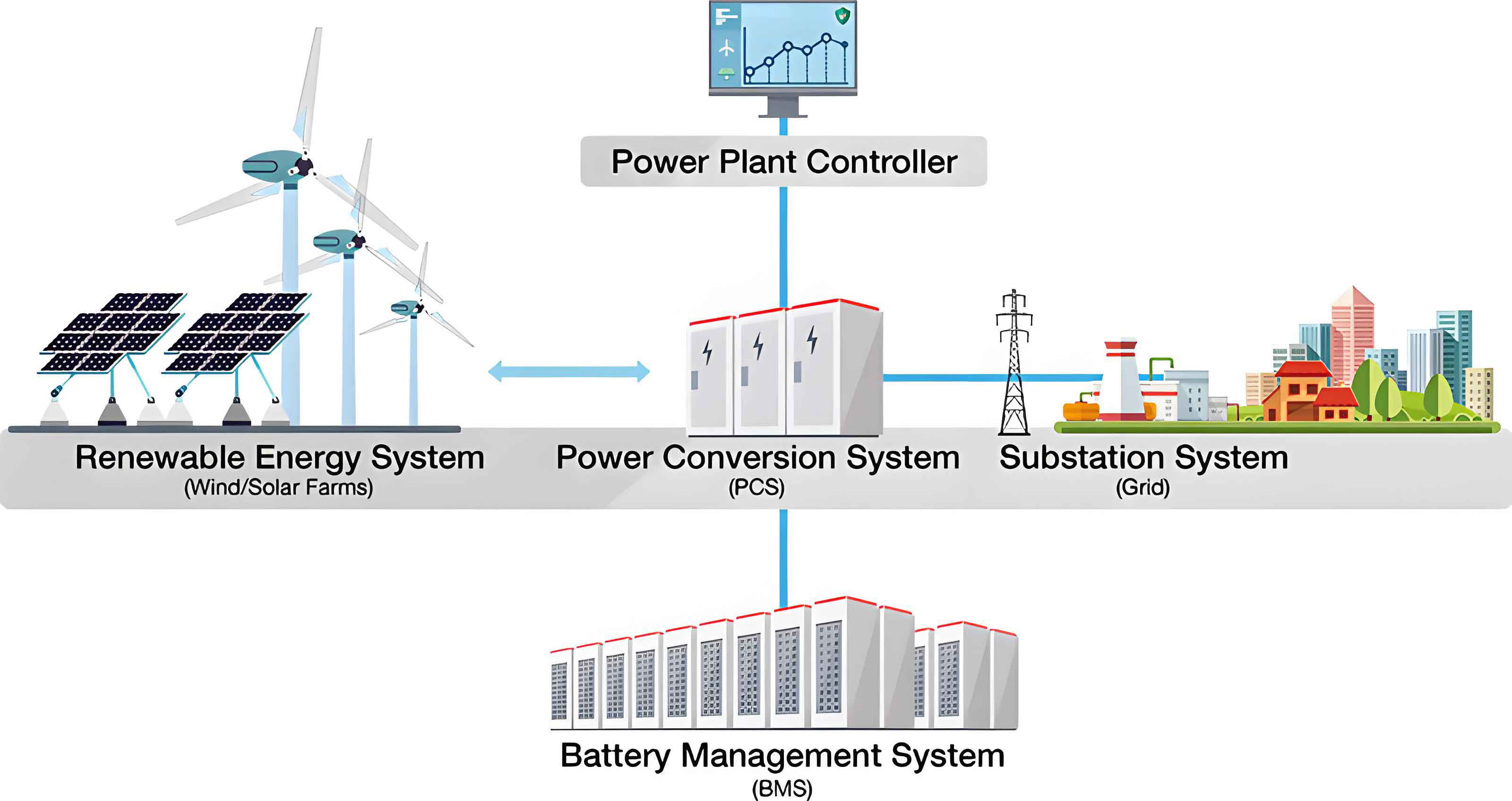
To simulate the real-world operation of a photovoltaic energy storage system (energy storage system) affected by series arc faults, a dedicated experimental platform is constructed. The platform mainly comprises a main circuit and a data acquisition module. The main circuit includes a photovoltaic array, a solar charge controller, batteries, and an arc fault generator. Figure 1 illustrates the schematic diagram of the photovoltaic energy storage system charging circuit. When the solar controller is conducting, the photovoltaic power source charges the battery. According to Kirchhoff’s Voltage Law (KVL), the arc voltage \(U_a\) can be expressed as:
$$U_a = E – U_b$$
where \(E\) is the electromotive force of the photovoltaic power source and \(U_b\) is the load voltage of the charging circuit. The photovoltaic array consists of 18 monocrystalline silicon modules, equally divided into 3 strings, with 6 modules per string. The main parameters of the PV modules are listed in Table 1.
| Parameter | Value |
|---|---|
| Pmax / W | 100 (1 ± 3%) |
| ISC / A | 7.78 |
| VOC / V | 22.49 |
| Im / A | 5.65 |
| Vm / V | 17.88 |
The solar charge controller (model ML60415F) is employed, which has a rated charging current of 60 A and a rated load current of 40 A. It features Maximum Power Point Tracking (MPPT) control technology, with a tracking efficiency exceeding 99.5%. This controller adopts a three-stage charging strategy: Constant-Current (C-C), Constant-Voltage (C-V), and Floating-Charge (C-F). Table 2 describes the characteristics of each stage.
| Charging stage | Voltage threshold | Operating characteristics |
|---|---|---|
| C-C | — | Constant maximum charging current, voltage increasing |
| C-V | 56.8 V | Constant maximum charging voltage, current gradually decreasing |
| C-F | 54.4 V | Small charging current, voltage reduced, maintaining full state |
The circuit utilizes four series-connected 6-EVF-32.2 batteries, each with a rated capacity of 32.2 Ah, rated voltage of 12 V, and rated charging current of 3.8 A. The series arc fault generator is designed according to the national standard GB/T 31143-2014 and IEC 62606. It consists of an insulating bracket, contacts, a sliding table, and a control circuit. In the experiments, the moving contact is a pointed copper rod with a diameter of 5 mm, while the stationary contact is a flat carbon rod with a diameter of 5 mm.
For data acquisition, an LHB150V5VT1 voltage transformer is used to measure the voltage signals across the arc generator electrodes and the PV array output. Its measurement range is 0–150 V with a frequency response from DC to 20 kHz and an accuracy of 0.2%. An LHB20A5VY2 Hall current transformer is employed to measure the loop current. This transformer has a measurement range of 0–50 A, a bandwidth from DC to 100 kHz, and an accuracy of 0.5%. Signals are digitized using a 16-bit analog-to-digital converter (NI-USB3200) data acquisition card and transmitted to a computer. The sampling frequency is set to 50 kHz.
Following the experimental scheme in Table 3, nine groups of experiments are conducted under different PV string numbers and battery charging states. In Table 3, “normal” refers to the state where the arc generator contacts are tightly closed, and “fault” refers to the state where an arc burns between the contacts. The experiments are conducted under irradiance of 440–460 Lux.
| Experiment No. | Charging stage | Branch | Working state |
|---|---|---|---|
| S1 | C-C | 1 | Normal / Fault |
| S2 | C-V | 1 | Normal / Fault |
| S3 | C-F | 1 | Normal / Fault |
| S4 | C-C | 2 | Normal / Fault |
| S5 | C-V | 2 | Normal / Fault |
| S6 | C-F | 2 | Normal / Fault |
| S7 | C-C | 3 | Normal / Fault |
| S8 | C-V | 3 | Normal / Fault |
| S9 | C-F | 3 | Normal / Fault |
2.2 Characteristic Analysis
The current and voltage waveforms under the three charging states exhibit distinct characteristics. In the C-C stage, the current is maximal among the three stages. In the C-V stage, the voltage reaches its maximum, and the current gradually decreases over time. In the C-F stage, a small current maintains the battery’s fully charged state. Significantly, the current waveform during the C-V stage shows more pronounced fluctuations when an arc fault occurs. The pulse peak-to-peak values are calculated for both normal and fault states across the different charging stages. Table 4 summarizes these findings—when a series arc fault occurs, the current pulse peak-to-peak values increase by more than 1.44 times compared to the normal state, whereas the voltage waveform changes are relatively smaller. This suggests that the current signal is more sensitive to series arc faults and is therefore selected as the identification signal for this study.
| State | C-C | C-V | C-F |
|---|---|---|---|
| P-P normal current / A | 0.23 | 0.29 | 0.28 |
| P-P fault current / A | 0.56 | 0.59 | 0.42 |
| P-P normal voltage / V | 7.58 | 8.96 | 8.88 |
| P-P fault voltage / V | 11.56 | 12.41 | 10.15 |
2.3 SVD-based Signal Denoising
In the actual operation of photovoltaic systems, the measured electrical signals are often affected by complex factors such as irradiance fluctuations, maximum power point variations of the solar controller, and electromagnetic noise. These factors introduce substantial spikes that can obscure the arc fault features. To enhance the noise immunity of the identification method, signal filtering is necessary. In this study, SVD is chosen for denoising due to its advantages of minimal information loss, controllable denoising degree, and high computational efficiency.
The SVD-based filtering method is implemented as follows:
(1) For an \(m \times n\) matrix \(A\), the singular value decomposition is given by:
$$A = U \Sigma V^{T}$$
with
$$\Sigma = diag(\sigma_1, \sigma_2, \dots, \sigma_r), \quad \sigma_i > 0 \quad (i = 1, \dots, r)$$
where \(U\) is an \(m \times m\) real symmetric matrix (left singular matrix), \(\Sigma\) is an \(m \times n\) matrix with singular values on its main diagonal arranged in descending order, and \(V\) is an \(n \times n\) real symmetric matrix (right singular matrix).
(2) The total singular value energy \(E\) is calculated as:
$$E = \sum_{i=1}^{r} \sigma_i^2$$
The energy contribution ratio \(E_i\) of each singular value is:
$$E_i = \frac{\sigma_i^2}{E}$$
Singular values with a cumulative contribution rate of at least 90% are retained, while the remaining singular values are set to zero, yielding matrix \(\Sigma^{*}\):
$$\Sigma^{*} = diag(\sigma_1, \sigma_2, \dots, \sigma_a, 0, \dots, 0), \quad \text{where} \quad \sum_{i=1}^{a} E_i \ge 0.9$$
(3) The denoised signal is reconstructed as:
$$A^{*} = U \Sigma^{*} V^{T}$$
Experimental results show that SVD filtering effectively removes glitches from current signals, making the normal current closer to an ideal straight line while preserving the fluctuations and spikes induced by series arc faults, as shown in Fig. 1.
2.4 Thermal Colormap Conversion
In practical PV energy storage systems, normal data are readily available, but acquiring series arc fault data is costly and time-consuming. This is particularly pronounced during the C-V and C-F stages, where charging times are short and current levels are low, resulting in unstable arcing and imbalanced sample sizes between normal and fault conditions. To overcome this issue, the one-dimensional time-series current data are converted into images using the ‘hot’ colormap scheme. Higher current values are mapped to brighter colors (white or yellow), while lower values are mapped to darker colors (black or dark red). This conversion provides a clear visual representation of data anomalies.
To validate the distinctiveness of the images, the Mean Squared Error (MSE) between thermal images of normal and fault states is computed. For each of the S1–S3 experimental groups, 100 current segments are extracted from both states, and the MSE is calculated as follows:
$$MSE = \frac{1}{mn}\sum_{i=0}^{m-1}\sum_{j=0}^{n-1}\left[I(i,j) – \hat{I}(i,j)\right]^2$$
where \(I\) is the reference normal image and \(\hat{I}\) is the comparison image. The results demonstrate that fault-state thermal images exhibit significantly larger MSE values relative to normal images, confirming the discriminative capability of the representation. However, some overlap remains, highlighting the need for a robust deep learning approach for automatic feature extraction and classification.
3. Fault Arc Recognition Model Architecture
3.1 Original ConvNeXt Architecture
ConvNeXt is a modern convolutional neural network architecture that builds upon residual networks by incorporating advanced techniques such as depthwise separable convolution, inverted bottlenecks, the GELU activation function, and layer normalization. Its key design choices include: (1) a patch-based stem layer using a stride-4 convolution to partition the input image into non-overlapping patches; (2) inverted bottleneck blocks that follow an expand–depthwise–reduce order to enhance information flow; (3) the replacement of standard convolution with depthwise separable convolution (DSC), which significantly reduces parameter count and computational cost; and (4) the use of GELU activation instead of ReLU, along with fewer activation layers, to preserve important feature information.
In DSC, each input channel is convolved with a single kernel, producing an output feature map with the same number of channels as the input. A subsequent \(1 \times 1\) pointwise convolution then fuses the channels and allows the output dimensionality to be adjusted. This approach dramatically reduces parameters relative to standard convolution while maintaining high computational efficiency. The depthwise separable convolution operation for an input feature map of size \(W \times H \times C\) with a kernel size of \(k \times k\) yields a parameter count of \(k^2 C\) and computational cost of \(k^2 C W’H’\), where \(W’\) and \(H’\) are the output dimensions.
3.2 GC-ConvNeXt: Improved Design
To further reduce the parameter count and facilitate deployment on embedded devices, the original ConvNeXt network is modified by incorporating Group Convolution (GConv) and Channel shuffle operations. GConv partitions the input channels into multiple groups, performing independent convolution within each group. This increases the diagonal correlation between filters, reduces the number of parameters, and has a regularization effect. For an input with \(C\) channels divided into \(g\) groups, each containing \(C/g\) channels, the parameter count becomes \(k^2 C\), which is \(g\) times fewer than standard convolution when generating the same number of output feature maps.
However, GConv prevents information exchange between channel groups. To address this limitation, the Channel shuffle operation is applied. This operation reshapes the output channels, transposes them, and then flattens them, effectively enabling cross-group information flow. Given four output feature maps of size \(56 \times 56 \times 32\), with a total of \(4 \times 32\) channels, the channels are first reshaped to (4, 32), then transposed, and finally flattened for the next layer. In the improved design, the input channels are divided into 4 groups, with 8 channels per group. This modification reduces the parameter count of the model by 33% compared to the original ConvNeXt.
3.3 Overall GC-ConvNeXt Model Architecture
The GC-ConvNeXt model processes input thermal colormap images of resolution \(224 \times 224\). The operational flow is as follows:
(1) The input undergoes standard convolution and depthwise convolution operations.
(2) The channel features are processed through GConv and Channel shuffle, with the input channels divided into 4 groups.
(3) A global average pooling layer computes the mean of each channel’s feature map, achieving dimensionality reduction.
(4) Fully connected layers classify the input samples.
To improve convergence speed and recognition accuracy, a Layer Scale operation is included. This multiplies the input feature layer by a trainable parameter vector, with the scaling factor initialized to \(1 \times 10^{-6}\).
3.4 Model Training
To ensure consistent dataset sizes, the data are segmented into unit time windows of 1024 sampling points (corresponding to 20.48 ms at a 50 kHz sampling rate). From experiments S1–S6 (the first two branches), 2000 normal and 1000 fault samples are extracted per experiment, yielding a total of 18000 samples. These samples are filtered using SVD and converted to thermal images, forming the Dataset. The dataset is split into training and validation sets in an 8:2 ratio. Dataset_CC, Dataset_CV, and Dataset_CF are constructed from the third branch (S7–S9) to evaluate generalization performance.
The model is trained using the TensorFlow framework on an AMD R7-6800H CPU (3.20 GHz). The categorical cross-entropy loss function is adopted:
$$Loss = -\frac{1}{n}\sum_{i=1}^{n}\sum_{j=1}^{m} y_{ij} \log(\hat{y}_{ij})$$
where \(n\) is the number of samples, \(m\) is the number of classes, \(y_{ij}\) is the actual label, and \(\hat{y}_{ij}\) is the predicted probability. SGD with momentum is selected as the optimizer:
$$v_{t+1} = \gamma v_t + \eta \nabla L(\theta_t)$$
$$\theta_{t+1} = \theta_t – v_{t+1}$$
where \(\eta\) is the learning rate, \(\gamma\) is the momentum coefficient (0.9), and \(v_t\) is the momentum at time \(t\). The cosine annealing scheduler is used to adjust the learning rate. The hyperparameters are: Epoch = 30, Batch size = 24, initial learning rate = 0.005. The model reaches a validation accuracy of 97.36% with a loss of 0.1072 after 30 epochs.
The comparison between the original ConvNeXt and the improved GC-ConvNeXt on key metrics is presented in Table 5.
| Model | Accuracy/% | Dataset_CC/% | Dataset_CV/% | Dataset_CF/% | Avg. generalization/% | Parameters |
|---|---|---|---|---|---|---|
| ConvNeXt | 97.31 | 95.25 | 96.15 | 95.80 | 95.73 | 10882 |
| GC-ConvNeXt | 97.36 | 95.60 | 96.20 | 96.15 | 95.98 | 6946 |
The improved model achieves a slightly higher recognition accuracy and 0.2% improvement in average generalization performance while reducing the parameter count by 33%, demonstrating its effectiveness and suitability for embedded deployment.
4. Data Augmentation for Imbalanced Fault Data
4.1 Traditional Data Augmentation
In practice, the number of fault samples is often far smaller than the number of normal samples, leading to imbalanced datasets and degraded model performance, particularly for minority classes. To mitigate this issue, traditional data augmentation techniques are first explored, including rotation, adding Gaussian noise, random cropping, and brightness adjustment. These methods are applied to the fault samples in the training set of the GC-ConvNeXt model. For each method, 4800 virtual fault samples are generated and combined with the original 4800 fault samples to balance the training set. Table 6 summarizes the dataset construction approach.
| Dataset split | Normal samples | Fault samples |
|---|---|---|
| Training set | 9600 | 4800 + 4800 (new virtual data) |
| Validation set | 2400 | 1200 |
The test results in Table 7 indicate that although the augmentations improve validation accuracy, most methods reduce generalization performance. Only the rotation method yields a slight improvement. This is attributed to the potential destruction of important structural features and image quality by these transformations, which prevents the model from effectively learning key discriminative information.
| Method | Accuracy/% | Dataset_CC/% | Dataset_CV/% | Dataset_CF/% | Avg. generalization/% |
|---|---|---|---|---|---|
| Baseline | 97.36 | 95.60 | 96.20 | 96.15 | 95.98 |
| Rotation | 97.39 | 95.70 | 96.20 | 96.35 | 96.08 |
| Noise | 97.47 | 95.35 | 95.90 | 95.80 | 95.69 |
| Crop | 97.56 | 94.95 | 95.80 | 95.50 | 95.42 |
| Brightness | 97.58 | 95.40 | 96.10 | 96.25 | 95.91 |
4.2 Mixup-based Data Augmentation
Mixup-based data augmentation methods, including Mixup, CutMix, and Manifold Mixup, overcome the limitations of single-sample augmentation by interpolating or fusing different samples to create virtual training data, thereby increasing sample diversity and improving the generalization of deep learning models.
(1) Mixup creates virtual training samples via convex combinations of training examples and their labels. For a pair of samples \((X_1, Y_1)\) and \((X_2, Y_2)\), the new sample \((\tilde{X}, \tilde{Y})\) is generated as:
$$\tilde{X} = \lambda X_1 + (1-\lambda) X_2$$
$$\tilde{Y} = \lambda Y_1 + (1-\lambda) Y_2$$
where \(\lambda \sim \text{Beta}(\alpha, \alpha)\). The parameter \(\alpha\) controls the interpolation strength. Smaller \(\alpha\) values increase the probability of \(\lambda\) being close to 0 or 1, producing samples that resemble one of the original samples. This linear relationship between samples and labels provides a strong regularization effect and improves model generalization.
(2) CutMix replaces a region of one image with a patch from another image instead of linearly interpolating pixels. The new sample is defined as:
$$\tilde{X} = M \odot X_1 + (1-M) \odot X_2$$
$$\tilde{Y} = \lambda Y_1 + (1-\lambda) Y_2$$
where \(M\) is a binary mask indicating the cropping region, and \(\lambda\) follows a Beta distribution. CutMix prevents the generation of uninformative blurred samples and enhances robustness against occlusion.
(3) Manifold Mixup performs mixing not only on input samples but also on hidden features in the feature space. In the GC-ConvNeXt architecture, the Manifold Mixup operation is applied at the output of the sixth layer (as shown in Fig. 1). For two input samples \(X_i\) and \(X_j\), the mixed feature is computed as:
$$\tilde{X}_{mix} = \lambda g_k(X_i) + (1-\lambda) g_k(X_j)$$
$$\tilde{Y}_{mix} = \lambda Y_i + (1-\lambda) Y_j$$
where \(g_k(\cdot)\) denotes the feature extraction up to the \(k\)-th layer. After mixing, the new sample continues the forward pass through the remaining layers. The loss is calculated using the mixed prediction and the mixed labels. During training, the mixing layer index \(k\) is selected randomly, which increases the model’s ability to learn richer representations.
This paper further proposes separating the mixing ratios of the sample space and the label space to better balance majority and minority classes. The label mixing is adjusted as:
$$\tilde{Y}_{mix}’ =
\begin{cases}
\tilde{Y}_{mix}, & \text{if } \lambda \in [\beta, 1-\beta] \\
Y_i, & \text{if } \lambda > \beta \text{ and } Y_i = [0,1] \\
Y_j, & \text{if } \lambda < [1-\beta] \text{ and } Y_j = [0,1]
\end{cases}
$$
where \(\beta\) is a threshold parameter. This allows the synthetic sample to be labeled as the minority class with a certain probability, effectively shifting the decision boundary towards the majority class and mitigating the class imbalance issue.
4.3 Performance Comparison of Data Augmentation Methods
The three mixup-based methods are evaluated using the GC-ConvNeXt model with the Dataset. The augmentation is applied only during training, while the validation set remains unchanged. The results are summarized in Table 8 and Table 9.
| Method | Validation accuracy/% |
|---|---|
| Baseline | 97.36 |
| Mixup | 97.81 |
| CutMix | 97.73 |
| Manifold Mixup (\(\beta=0.8\)) | 97.83 |
| Method | Dataset_CC/% | Dataset_CV/% | Dataset_CF/% | Avg. generalization/% |
|---|---|---|---|---|
| Baseline | 95.60 | 96.20 | 96.15 | 95.98 |
| Mixup | 95.80 | 96.45 | 96.25 | 96.17 |
| CutMix | 95.40 | 96.20 | 95.90 | 95.83 |
| Manifold Mixup | 95.95 | 96.70 | 96.85 | 96.50 |
The Manifold Mixup method with \(\beta = 0.8\) achieves the best performance, delivering both the highest validation set accuracy (97.83%) and the highest average generalization accuracy (96.50%). This optimal model is denoted as MIX-GC-ConvNeXt. The improved performance can be attributed to its ability to augment data in the feature space, which increases sample diversity and helps the model learn more generalizable features, thus alleviating the class imbalance issue effectively.
5. Recognition Performance Evaluation
5.1 Prediction Scatter Plot Analysis
To gain deeper insights into the model’s predictive behavior, the raw output scores for both classes (normal and fault) are visualized as scatter plots. The center coordinates of the predicted clusters for each model are calculated and presented in Table 10.
| Model | Normal center | Fault center | Distance |
|---|---|---|---|
| ConvNeXt | (3.35, -2) | (0.18, 4.1) | 6.87 |
| GC-ConvNeXt | (2.43, -1.85) | (-1.69, 5.19) | 8.18 |
| MIX-GC-ConvNeXt | (1.81, -0.9) | (-0.03, 2) | 1.47 |
The GC-ConvNeXt model shows a larger distance between cluster centers compared to the original ConvNeXt, suggesting that the group convolution operation enhances the model’s ability to distinguish between different classes. In contrast, Manifold Mixup in the MIX-GC-ConvNeXt model brings the cluster centers closer together due to the interpolation of features and labels, effectively smoothing the decision boundary. Despite the reduced class separation in the scatter plot, the model’s accuracy improves, indicating that the smoothing leads to better generalization.
5.2 Recall and F1 Score Analysis
To comprehensively evaluate the classification performance, the confusion matrix is constructed for each model on the combined Dataset_CC, Dataset_CV, and Dataset_CF, comprising 6000 samples. Recall and F1 scores are computed as follows:
$$\text{Recall} = \frac{TP}{TP + FN}$$
$$\text{Precision} = \frac{TP}{TP + FP}$$
$$F1 = 2 \times \frac{\text{Precision} \times \text{Recall}}{\text{Precision} + \text{Recall}}$$
The results are summarized in Table 11.
| Model | Recall/% | F1 score |
|---|---|---|
| ConvNeXt | 91.87 | 0.956 |
| GC-ConvNeXt | 92.57 | 0.958 |
| MIX-GC-ConvNeXt | 93.40 | 0.964 |
Both the recall and F1 scores progressively improve from ConvNeXt to GC-ConvNeXt to MIX-GC-ConvNeXt, demonstrating that the combination of architectural improvements and mixup-based data augmentation significantly enhances the model’s fault detection capability.
5.3 Robustness Testing
5.3.1 Solar Charge Controller Startup Impact
During the startup of the solar charge controller, the current in the battery charging circuit gradually increases with large fluctuations. To evaluate the model’s robustness against such transients, 200 current segments are extracted from startup signals, creating the Dataset_start. The MIX-GC-ConvNeXt model correctly classifies all 200 samples without any misjudgment, confirming its strong robustness to controller startup transients.
5.3.2 Noise Interference Testing
To simulate realistic noise environments, Gaussian white noise with varying signal-to-noise ratios (45 dB, 40 dB, 35 dB, 30 dB, 25 dB, 20 dB) is added to the current signals. The Dataset_S_test is created using SVD filtering followed by thermal image conversion, while Dataset_NS_test is created without filtering. Table 12 reports the recognition accuracy under different noise intensities. The results indicate that SVD filtering markedly enhances the model’s noise immunity. When the SNR is not lower than 30 dB, the model achieves accurate recognition of over 90%. Even at 25 dB, the filtered model maintains an 88.01% recognition rate, significantly outperforming the unfiltered model (87.36%).
| Dataset | SVD | 45 dB/% | 40 dB/% | 35 dB/% | 30 dB/% | 25 dB/% |
|---|---|---|---|---|---|---|
| Dataset_S_test | Yes | 96.22 | 95.36 | 93.31 | 91.46 | 88.01 |
| Dataset_NS_test | No | 93.66 | 92.11 | 90.96 | 88.96 | 87.36 |
At an SNR of 35 dB, the scatter plot illustrates the impact of SVD filtering on classification. Without SVD filtering, a significant number of fault samples are misclassified into the normal cluster (90.96% accuracy), whereas after SVD filtering, the misclassifications are notably reduced (93.31% accuracy). These results validate the necessity and effectiveness of the SVD-based preprocessing approach.
5.4 Runtime Performance
Timely detection is critical for effective arc fault protection. According to the standard GB/T 39750-2021, the protective device should extinguish the arc before the arc energy exceeds 750 J or the arc duration exceeds 2.5 s, whichever comes first. The runtime test indicates that the average processing time per sample, including preprocessing and model inference, is less than 22 ms, providing sufficient time for the circuit breaker to isolate the faulty circuit.
5.5 Comparison with Wavelet Domain Filtering
A comparative study is conducted between the proposed SVD filtering method and the commonly used wavelet packet threshold filtering method. The comparison focuses on recognition accuracy, generalization, and anti-interference performance at 35 dB SNR under the MIX-GC-ConvNeXt model. The results are shown in Table 13.
| Filtering method | Accuracy/% | Generalization/% | 35 dB anti-interference/% |
|---|---|---|---|
| Wavelet packet | 96.2 | 92.58 | 92 |
| SVD (proposed) | 97.83 | 96.5 | 93.31 |
For the wavelet packet filtering method, the recognition accuracy of normal samples is only 93.79%, compared to 99.6% for SVD filtering. The wavelet packet filtering introduces some spikes in normal signals as visible in the transformed images, leading to misclassifications. Therefore, the SVD-based denoising approach demonstrates superior overall performance for this application.
5.6 Comparison with State-of-the-Art Methods
The proposed MIX-GC-ConvNeXt is compared with several existing fault arc identification methods, including wavelet energy entropy with extreme learning machine (ELM), standard convolutional neural network (CNN), and Gramian Angular Summation Field (GASF) with LeNet-5. The same dataset configurations are used across all methods. Table 14 presents the comparative results.
| Method | Accuracy/% | Generalization/% | 35 dB anti-interference/% |
|---|---|---|---|
| Wavelet energy entropy + ELM | 92.78 | 67.85 | 61.42 |
| CNN | 94.92 | 78.61 | 65.90 |
| GASF + LeNet-5 | 96.17 | 86.31 | 77.30 |
| MIX-GC-ConvNeXt (proposed) | 97.83 | 96.50 | 93.31 |
The proposed method significantly outperforms the other approaches in all three metrics. Notably, it achieves a generalization accuracy of 96.50%, which is more than 10 percentage points higher than the GASF+LeNet-5 method, demonstrating its superior ability to adapt to unseen operating conditions. The excellent anti-interference performance further confirms the effectiveness of the integrated SVD filtering and MIX-GC-ConvNeXt architecture for series arc fault identification in photovoltaic energy storage systems.
6. Conclusion and Outlook
This paper conducted a systematic investigation into the identification of series arc faults in the charging circuits of photovoltaic energy storage systems. The main contributions and conclusions are summarized as follows:
(1) A dedicated experimental platform was constructed to simulate series arc faults in PV battery charging circuits. The current signal was identified as the most suitable identification signal due to its higher sensitivity to arc faults. The application of SVD filtering effectively reduced the noise interference from various sources while preserving the key fluctuation features induced by series arc faults, thereby significantly enhancing the noise immunity of the identification method.
(2) An improved ConvNeXt network model, named GC-ConvNeXt, was proposed. By integrating GConv and Channel shuffle operations, the model achieved a 33% reduction in parameter count while maintaining high recognition accuracy (97.36%) and improving generalization performance by 0.2%. The reduced parameter count facilitates deployment on embedded devices.
(3) To address the sample imbalance problem commonly encountered in fault arc experiments, traditional and mixup-based data augmentation methods were compared. The results indicated that traditional methods may lead to feature information loss and image quality degradation, while mixup-based methods effectively increase data diversity and enhance model generalization. The Manifold Mixup method, which separates the mixing ratios of sample space and label space, achieved the best performance. The final optimal model, MIX-GC-ConvNeXt, incorporates this enhanced Manifold Mixup method.
(4) Through scatter plot analysis, the GConv improvement enhanced the model’s ability to distinguish between different classes, while Manifold Mixup improved generalization by smoothing decision boundaries. The recall and F1 scores progressively improved, confirming the effectiveness of the proposed approach. Robustness tests demonstrated that the optimal model maintains stable and reliable performance under solar charge controller startup and noise interference conditions. When the SNR is not lower than 30 dB, the model achieves over 90% recognition accuracy.
(5) Comparative studies showed that the proposed SVD filtering method outperforms the commonly used wavelet packet threshold filtering method in terms of recognition accuracy, generalization ability, and anti-interference performance. The MIX-GC-ConvNeXt model achieves superior performance compared to other existing fault arc identification methods across all evaluation metrics. The runtime for a single sample is less than 22 ms, meeting the real-time identification requirements.
Future work will focus on the following directions: First, investigating fault arcs at the rear end of the solar charge controller and developing advanced identification methods that can recognize series arc faults at different locations by monitoring only the PV array output current. Second, developing hardware systems for arc fault identification algorithms, aiming to create arc fault circuit breakers specifically designed for PV energy storage system battery charging circuits, thereby enabling fast and effective fault arc interruption in practical applications.