
In the context of the global energy transition and the “dual carbon” goal, new energy microgrids have emerged as one of the most promising forms of integrating distributed renewable energy sources such as photovoltaic generation and wind power. However, the inherent stochastic nature and volatility of these renewable sources impose severe challenges on the real-time power balance, voltage regulation, and frequency stability of microgrids. After a thorough analysis of the existing technical bottlenecks, I firmly believe that the energy storage system serves as the critical enabling technology to overcome these obstacles. In this paper, I focus on two fundamental problems: the optimal configuration strategy of the energy storage system and its cooperative control method. I first discuss how to design the capacity and power rating of the energy storage system from the perspectives of economics, reliability, and uncertainty. Then, I investigate hierarchical control, multi-agent based distributed control, and model predictive control approaches in detail. Finally, I explore the coupling relationship between configuration and control, and present an outlook on future development trends, aiming to provide theoretical support for the planning and efficient operation of new energy microgrids.
1. Structure and Core Role of the Energy Storage System in New Energy Microgrids
Before diving into the configuration and control details, I would like to clarify the typical architecture of a new energy microgrid. A microgrid is a hybrid power generation and distribution system composed of distributed generators, energy storage devices, power conversion units, loads, and monitoring protection devices. Its defining characteristic is the use of renewable energy sources such as photovoltaic modules and wind turbines as the primary generating units. From a physical standpoint, a microgrid is connected to the upstream main grid through a point of common coupling (PCC). It can operate in grid-connected mode or islanded mode. In grid-connected mode, the microgrid exchanges power with the main grid and can participate in peak shaving and frequency regulation as a controlled entity. In islanded mode, the microgrid must independently maintain internal power balance as well as voltage and frequency stability, which places extremely high demands on the coordination of the internal control system.
In my opinion, the energy storage system occupies the central position in the microgrid due to its rapid response capability and flexible regulation characteristics. On one hand, the energy storage system can achieve peak shaving and energy time-shifting: when renewable generation exceeds the local load demand, the surplus electricity is stored instead of being wasted; when the load is high or the renewable output is low, the stored energy is released to support the supply. This smooths the net load curve, reduces dependence on the main grid, and decreases the number of start-ups of backup generators. On the other hand, the energy storage system is able to provide fast power support and virtual inertia during system disturbances. By absorbing or injecting active power almost instantaneously, it suppresses severe voltage and frequency excursions and improves the dynamic stability of the entire microgrid.
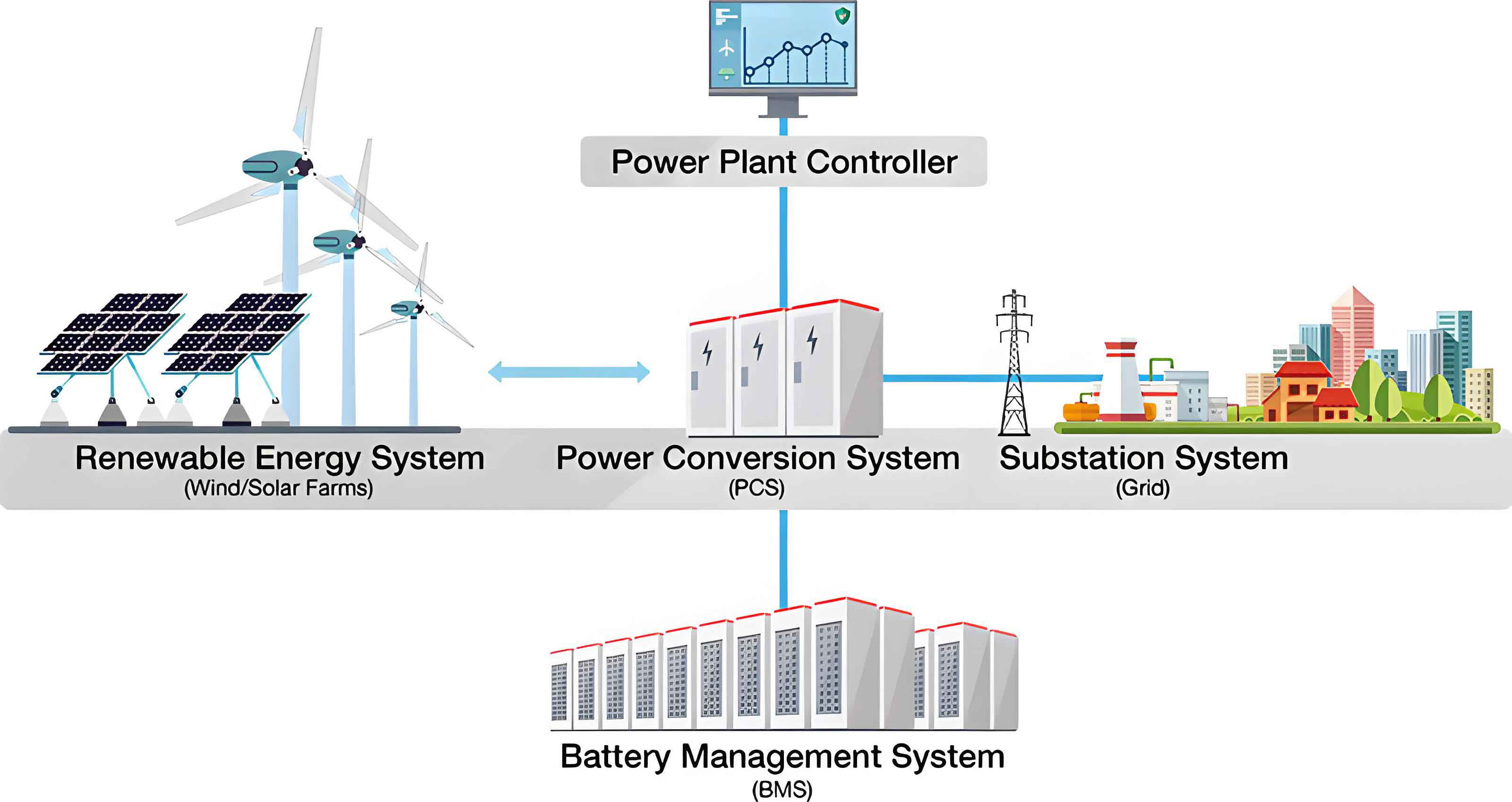
To systematically summarize the roles and functions of each microgrid component, I have constructed the following table. This table provides a clear overview of the functionality that each unit contributes to the operation of the new energy microgrid.
| Component | Primary Function | Interaction with Energy Storage System |
|---|---|---|
| Photovoltaic panels | Convert sunlight into DC electricity | Output power depends on irradiance and temperature; storage compensates for fluctuations |
| Wind turbines | Convert wind kinetic energy into electrical power | Variable output due to wind speed; storage smooths rapid changes |
| Energy storage system | Absorb, store, and release electrical energy | Acts as the balancing source between generation and consumption |
| Power conversion system | Interface between AC/DC buses and generators, storage, and loads | Controls the charging/discharging power of the storage system |
| Loads | Consume electrical energy | Storage meets peak load requirements and supports uninterruptible power |
| Main grid connection (PCC) | Connects microgrid to external grid | Storage enables islanded operation when the PCC is disconnected |
2. Optimal Configuration Strategies for the Energy Storage System
The configuration of an energy storage system determines its rated power, rated capacity, and often the selection of multiple storage technologies. This is the most fundamental design decision because it largely defines the investment cost, operational flexibility, and reliability of the entire microgrid. Based on my review of current research and engineering practice, I categorize the configuration strategies into three major groups: economic optimization, multi-objective reliability-economy optimization, and hybrid energy storage system configuration. Each of these approaches has its own mathematical formulation, solution methods, and engineering applicability.
2.1 Economic Optimization Method for Energy Storage Capacity Configuration
The primary objective in the economic configuration method is to minimize the total life-cycle cost of the system while ensuring that the basic operational constraints are satisfied. In recent years, I have noticed that many studies formulate this problem as a mixed-integer linear programming or nonlinear programming model. The total cost typically includes the initial investment cost of the storage system, the operation and maintenance cost, replacement costs, and the cost of power exchanged between the microgrid and the main grid. Let me define the following decision variables:
Let \(P_{ESS}(t)\) be the charging/discharging power of the energy storage system at time \(t\). Positive \(P_{ESS}(t)\) indicates discharging, and negative indicates charging. Let \(E_{ESS}(t)\) be the state of energy stored in the battery. The capacity to be optimized is \(E_{cap}\), and the rated power is \(P_{cap}\). The total annual cost function can be expressed as:
$$C_{total} = C_{inv} + C_{om} + C_{rep} + C_{grid}$$
where:
$$C_{inv} = c_e E_{cap} + c_p P_{cap}$$
In this expression, \(c_e\) denotes the cost per unit energy capacity (\$/kWh), and \(c_p\) denotes the cost per unit power rating (\$/kW). The operation and maintenance cost over a year is often modeled as a fixed fraction of the initial investment:
$$C_{om} = k_{om} C_{inv}$$
where \(k_{om}\) is the annual operation and maintenance coefficient. The replacement cost depends on the battery cycle life and the depth-of-discharge operation pattern. If the battery lifetime in years is \(Y_{bat}\), then the annualized replacement cost can be formulated as:
$$C_{rep} = \frac{C_{inv}}{Y_{bat}} r_d$$
where \(r_d\) is the discount factor. The grid exchange cost is:
$$C_{grid} = \sum_{t=1}^{T} \left[ \lambda_{buy}(t) P_{buy}(t) \Delta t – \lambda_{sell}(t) P_{sell}(t) \Delta t \right]$$
Here, \(\lambda_{buy}(t)\) and \(\lambda_{sell}(t)\) are the purchasing and selling prices of electricity at time \(t\), \(P_{buy}(t)\) and \(P_{sell}(t)\) denote the power imported from and exported to the main grid, respectively, and \(\Delta t\) is the time step duration. The overall objective is then:
$$\min_{E_{cap}, P_{cap}} C_{total}$$
subject to a set of constraints. The power balance constraint is:
$$P_{load}(t) = P_{DG}(t) + P_{ESS}(t) + P_{grid}(t)$$
where \(P_{load}(t)\) is the load demand, \(P_{DG}(t)\) is the distributed generation output, and \(P_{grid}(t)\) is the net power exchange with the main grid. The state-of-charge (SOC) dynamics of the energy storage system are defined as:
$$SOC(t+1) = SOC(t) + \frac{\eta_c P_{ESS}^{ch}(t) \Delta t}{E_{cap}} – \frac{P_{ESS}^{dis}(t) \Delta t}{\eta_d E_{cap}}$$
where \(P_{ESS}^{ch}(t)\) and \(P_{ESS}^{dis}(t)\) represent charging and discharging power levels, \(\eta_c\) and \(\eta_d\) are charging and discharging efficiencies, respectively. The state of charge is constrained between lower and upper limits:
$$SOC_{min} \le SOC(t) \le SOC_{max}$$
and the charging/discharging power is constrained by the rated power:
$$-P_{cap} \le P_{ESS}(t) \le P_{cap}$$
In practice, I have found that particle swarm optimization, genetic algorithms, and mixed-integer linear programming solvers are commonly used to obtain the globally optimal or near-optimal solutions for this model. This economic method is straightforward and well-established, but it heavily relies on the accuracy of the forecasted renewable generation and load data. It also has a tendency to under-size the storage capacity because extreme but rare operating scenarios are often omitted.
2.2 Multi-objective Configuration Considering Reliability and Economy
For critical loads such as hospitals, data centers, and industrial facilities, the sole objective of minimizing cost is no longer sufficient. In these scenarios, I emphasize the need for a multi-objective optimization framework that takes both reliability and economic performance into account. The reliability indicators commonly used in microgrid planning are the Loss of Load Probability (LOLP) and Expected Energy Not Supplied (EENS). These indicators capture the frequency and severity of power supply shortages. The mathematical definitions are as follows:
$$LOLP = \frac{1}{T} \sum_{t=1}^{T} I_{t}$$
where \(I_{t}\) is an indicator variable that equals 1 if the available generation plus storage cannot satisfy the load demand at time \(t\), and 0 otherwise. The EENS is defined as:
$$EENS = \sum_{t=1}^{T} \left[ P_{load}(t) – P_{avail}(t) \right] \Delta t, \quad \forall t \text{ with } P_{load}(t) > P_{avail}(t)$$
where \(P_{avail}(t)\) is the maximum available power from generation and storage at time \(t\). In the multi-objective configuration model, the optimization problem can be formulated as:
$$\min_{E_{cap}, P_{cap}} \left[ C_{total}, EENS \right]$$
or, equivalently, as a weighted sum:
$$\min \left( w_1 C_{total} + w_2 EENS \right)$$
subject to the same operational constraints described in the previous section. However, it is more informative to generate the Pareto optimal set rather than combining the objectives with fixed weights. Mathematically, a Pareto optimal solution is one in which any improvement in one objective causes a deterioration in at least one other objective. I can solve the multi-objective problem using the \(\epsilon\)-constraint method, non-dominated sorting genetic algorithm (NSGA-II), or multi-objective particle swarm optimization. The resulting Pareto front provides a range of compromise solutions. Decision-makers can then select the final configuration based on their risk preference and budget.
I have summarized the main differences between the economic-only and multi-objective configuration approaches in the following table.
| Aspect | Economic-only configuration | Multi-objective configuration |
|---|---|---|
| Objective | Minimize total life-cycle cost | Minimize cost and reliability indicators concurrently |
| Reliability metrics | Not explicitly modeled | LOLP, EENS, or system average interruption frequency |
| Solution method | MILP, GA, PSO | NSGA-II, \(\epsilon\)-constraint, weighted sum |
| Output | Single optimal solution | Pareto optimal set |
| Application areas | Grid-connected microgrids with low reliability requirements | Islanded microgrids with critical loads |
2.3 Hybrid Energy Storage System Optimal Configuration
In practice, I observe that no single type of energy storage technology can simultaneously satisfy the high energy density and high power density requirements of a new energy microgrid. Energy-type storage, such as lithium-ion batteries, has a high energy density but suffers from shortened lifetime when subjected to frequent high-power charge/discharge cycles. Power-type storage, such as supercapacitors, has excellent power density and long cycle life, but its energy density is low and its cost per kWh is relatively high. To circumvent this limitation, I strongly advocate the use of a hybrid energy storage system (HESS), which combines two or more storage technologies to exploit their complementary strengths. A typical HESS in a microgrid consists of a battery pack and a supercapacitor bank. The supercapacitor handles the high-frequency components of power fluctuations, thus protecting the battery from stress, while the battery deals with the low-frequency and sustained energy shifts.
The configuration of a HESS is more complex than that of a single storage system because it must not only decide the capacity of each storage unit, but also design a power-splitting strategy between them. One commonly used approach is to decompose the required compensation power \(P_{comp}(t)\) into low-frequency and high-frequency parts via a low-pass filter. Let \(\alpha\) be the filter time constant. The battery power is given by:
$$P_{bat}(t) = \frac{1}{1 + \tau s} P_{comp}(t)$$
where \(s\) is the Laplace operator, while the supercapacitor power is the residual:
$$P_{sc}(t) = P_{comp}(t) – P_{bat}(t)$$
The life consumption of the battery is strongly affected by the number of cycles and the depth of discharge. I can model the battery life degradation using the following simplified expression:
$$L_{bat} = \frac{1}{N_{cycle}} \sum_{i=1}^{N_{cycle}} \left( \frac{DOD_i}{DOD_{ref}} \right)^k$$
where \(L_{bat}\) is the battery lifetime loss, \(DOD_i\) is the depth of discharge of the \(i\)-th cycle, \(DOD_{ref}\) is the reference depth of discharge, and \(k\) is the exponent determined by the battery chemistry. The overall optimization objective for the HESS configuration can then be expressed as:
$$\min_{E_{bat}, P_{bat}, E_{sc}, P_{sc}, \tau} \left( C_{invest} + C_{om} + C_{replacement} + C_{penalty} \right)$$
subject to the dynamic constraints for each storage unit and the power balance. I also need to ensure that the state of charge of both the battery and supercapacitor remain within their allowable ranges:
$$SOC_{bat}^{min} \leq SOC_{bat}(t) \leq SOC_{bat}^{max}$$
$$SOC_{sc}^{min} \leq SOC_{sc}(t) \leq SOC_{sc}^{max}$$
To present the characteristics of different storage technologies and their roles in a HESS, I have produced the following comparison table.
| Storage Type | Energy Density | Power Density | Cycle Life | Cost per kWh | Primary Role in HESS |
|---|---|---|---|---|---|
| Lithium-ion battery | High | Medium | 2,000-5,000 cycles | Medium | Energy time-shifting, low-frequency power smoothing |
| Supercapacitor | Low | Very high | > 500,000 cycles | High | High-frequency transient absorption, protection of battery |
| Flow battery | Medium | Low | Very long | Long-term storage | Long-duration energy management |
| Flywheel | Low | High | Very long | High | Rapid frequency response and inertial support |
3. Cooperative Control Technology of the Energy Storage System in Microgrids
Once the energy storage system is sized and installed, the next critical issue is how to control it in real time so that the designed benefits can be fully realized. The control architecture of a microgrid determines how the storage system interacts with other distributed generators, loads, and the main grid. In my research, I have identified three major control directions: hierarchical control, multi-agent based distributed cooperative control, and model predictive control in the energy management system. These methods are not mutually exclusive; in fact, modern microgrids often integrate them to achieve both fast dynamic response and optimal economic dispatch.
3.1 Hierarchical Control Architecture
Hierarchical control is currently the most widely applied control architecture in microgrids. It is generally divided into three levels: primary control (bottom level), secondary control (middle level), and tertiary control (top level). I will describe each level in the context of the energy storage system. The primary control is the device-level autonomous control, which relies only on local measurements. For an energy storage inverter, the most common primary control strategy is droop control or virtual synchronous generator (VSG) control. The active power-frequency droop characteristic can be expressed as:
$$f = f_{ref} – m_p (P_{ESS} – P_{ref})$$
where \(f\) is the actual microgrid frequency, \(f_{ref}\) is the reference frequency, \(m_p\) is the droop coefficient for active power, \(P_{ESS}\) is the measured active power output of the storage unit, and \(P_{ref}\) is the reference active power set by the upper controller. Similarly, the voltage-reactive power droop control is:
$$V = V_{ref} – n_q (Q_{ESS} – Q_{ref})$$
where \(V\) is the terminal voltage, \(V_{ref}\) is the reference voltage, \(n_q\) is the reactive power droop coefficient, \(Q_{ESS}\) is the measured reactive power, and \(Q_{ref}\) is the reactive power reference. The primary control does not require communication and can stabilize the voltage and frequency within milliseconds.
The secondary control, on the other hand, uses a communication network to collect information from different local controllers and correct the steady-state deviations introduced by the primary control. For example, the secondary control restores the system frequency and voltage to their rated values. In addition, the secondary control can implement state-of-charge (SOC) equalization among multiple energy storage units. If multiple batteries are connected in parallel, the SOC balancing law can be designed as:
$$\Delta f_i = -m_p P_{ESS,i} + k_{SOC} (SOC_i – \overline{SOC})$$
where \(SOC_i\) is the state of charge of unit \(i\), \(\overline{SOC}\) is the average SOC of all units, and \(k_{SOC}\) is the equalization coefficient. This ensures that all storage units reach similar SOC levels during operation, thereby preventing over-charge or over-discharge of a single unit.
The tertiary control belongs to the energy management level. It is responsible for the economic optimal operation of the whole microgrid over a look-ahead horizon, such as 24 hours. Based on the forecast of renewable generation, load demand, and electricity tariff information, the tertiary control generates the optimal dispatch schedule for the energy storage system. The scheduling problem can be formulated as a linear or nonlinear optimization problem, and the resulting power commands are passed down to the secondary and primary controllers. I have summarized the three control levels in the following table.
| Control Level | Time Scale | Communication Requirement | Main Functions | Storage System Involvement |
|---|---|---|---|---|
| Primary control | Milliseconds to seconds | None (local measurement) | Voltage/frequency stabilization, power sharing | Droop or VSG control of storage inverters |
| Secondary control | Seconds to minutes | Low-bandwidth communication | Restore frequency/voltage, SOC equalization | Compensation signals for storage units |
| Tertiary control | Minutes to hours | Full communication with EMS | Economic dispatch, peak shaving, grid interaction | Optimal charging/discharging schedules |
3.2 Distributed Cooperative Control Based on Multi-Agent System
As the number of distributed units in a microgrid increases, the traditional centralized control architecture suffers from the curse of dimensionality and vulnerability to single-point failures. To address this issue, I have studied the multi-agent system (MAS) approach, which offers a more scalable and robust alternative. In the MAS framework, each distributed generator, energy storage unit, and controllable load is modeled as an agent that possesses computation, communication, and decision-making capabilities. The agents exchange local information with their neighboring agents through a sparse communication network and use a consensus algorithm to achieve a global control objective.
For the energy storage system in a microgrid, the goal of the multi-agent cooperative controller is to ensure that the total power demand is shared among all storage units in proportion to their capacities and that their SOC values are balanced. A typical first-order consensus algorithm for the storage units can be written as:
$$\dot{x}_i(t) = \sum_{j \in N_i} a_{ij} \left( x_j(t) – x_i(t) \right)$$
where \(x_i(t)\) is the state of the \(i\)-th agent (for example, its output power or SOC), \(N_i\) is the set of neighbors of agent \(i\), and \(a_{ij}\) are the elements of the adjacency matrix of the communication graph. If the graph is connected, the consensus algorithm guarantees that all states converge to the same value, i.e., \(x_i(t) \to x_{avg}\). For SOC balancing, the state \(x_i\) can be the normalized SOC:
$$x_i = SOC_i – \frac{1}{n} \sum_{j=1}^{n} SOC_j$$
Then the consensus algorithm adjusts the power references of each storage unit to drive \(x_i\) to zero. One of the most useful consensus-based control laws for storage units is:
$$P_{ESS,i}^{ref}(t) = \frac{SOC_i(t)}{\sum_{j \in G} SOC_j(t)} P_{total}^{ref}(t)$$
where \(P_{total}^{ref}(t)\) is the total required power from all storage units, and \(G\) is the set of all storage agents. This proportional sharing based on SOC ensures that each unit discharges in proportion to its available energy, which naturally prevents some units from being exhausted earlier than others.
The table below compares centralized control, decentralized control, and distributed multi-agent control in terms of several key performance indicators. This comparison helps me illustrate why distributed control is becoming more attractive for large-scale microgrids.
| Feature | Centralized control | Decentralized control | Distributed MAS control |
|---|---|---|---|
| Communication structure | Star topology with central controller | No communication between units | Sparse peer-to-peer network |
| Scalability | Poor for large number of units | Good but lacks global coordination | Excellent |
| Tolerance to single-point failure | Low (central controller failure causes total shut-down) | High | High |
| Global optimality | Can achieve if configured properly | Not guaranteed | Approaches global optimal through consensus |
| Computation burden | Very high at central station | Low | Distributed among agents |
3.3 Model Predictive Control in Energy Management System
In the energy management layer, I have found that model predictive control (MPC) is particularly powerful because it can handle system constraints and uncertainties in a systematic way. MPC is a closed-loop optimization strategy that repeatedly solves a finite-horizon optimal control problem based on the current state measurement and future predictions. In the context of the energy storage system, the MPC-based energy management has the following structure. At each sampling instant \(k\), the controller measures the current SOC of the storage system and obtains the forecast of photovoltaic output, wind power, and load demand over the prediction horizon \(N_p\). It then solves the following optimization problem:
$$\min_{\mathbf{P}_{ESS}} \sum_{t=k}^{k+N_p-1} \left( c_{op}(t) + c_{SOC}(t) + c_{pv}(t) \right)$$
where \(c_{op}(t)\) is the operation cost, \(c_{SOC}(t)\) penalizes SOC deviations from a reference value, and \(c_{pv}(t)\) penalizes curtailment of renewable generation. The decision vector \(\mathbf{P}_{ESS} = [P_{ESS}(k), P_{ESS}(k+1), \ldots, P_{ESS}(k+N_p-1)]\) contains the charging/discharging power values for the storage system over the prediction horizon. The optimization is subject to the same SOC dynamics and power constraints as in the configuration problem, but in discrete time:
$$SOC(k+1) = SOC(k) + \frac{\eta_c P_{ch}(k) \Delta t}{E_{cap}} – \frac{P_{dis}(k) \Delta t}{\eta_d E_{cap}}$$
Rather than implementing the entire optimal sequence, only the first control action \(P_{ESS}(k)\) is applied to the storage system. At the next sampling instant, the optimization is repeated with the updated forecast and measured state. This rolling horizon mechanism provides feedback correction and robustness against forecast errors.
I can further strengthen the MPC approach by integrating it with the multi-agent consensus algorithm discussed in the previous section. In this combined framework, the MPC is used at the tertiary level to generate optimal power setpoints of the whole microgrid, while the consensus algorithm is used at the secondary level to distribute the power commands among multiple storage agents in a distributed manner. The overall optimization problem for the coordinated MPC-consensus control can be formulated as:
$$\min \sum_{i=1}^{n} J_i(P_{ESS,i}, SOC_i) + \lambda \sum_{i=1}^{n} \sum_{j \in N_i} \left\| P_{ESS,i} – P_{ESS,j} \right\|^2$$
where \(\lambda\) is a weighting factor that penalizes disagreement among the neighboring agents. This hybrid approach has been shown to significantly improve the real-time response capability of distributed control while preserving the economic optimality of centralized MPC.
4. Coupled Optimization of Configuration and Cooperative Control
In traditional engineering practice, the configuration of the energy storage system and the design of its control strategy are carried out in a sequential manner. One first determines the capacity and power ratings based on a simplified operational scenario, and afterward develops a controller to operate the storage system. In my analysis, this sequential approach often leads to suboptimal solutions. The reason is that the optimal configuration depends on the control strategy that will be applied after installation; a control strategy with poor coordination may require a larger or smaller storage capacity to achieve the same performance. Conversely, the best control strategy cannot be designed without knowing the physical limits of the storage system. Therefore, I believe that configuration and control must be jointly optimized.
This coupled optimization problem can be formulated as a bi-level programming model. In the upper-level problem, the decision variables are the storage rated power and capacity. In the lower-level problem, the system operation is simulated under a selected control strategy, and the annual operating cost and reliability indicators are computed. The upper-level objective is to minimize the total life-cycle cost, while the lower-level objective is to minimize the daily operating cost subject to the energy storage constraints. Mathematically, the bi-level optimization can be represented as:
$$\min_{E_{cap}, P_{cap}} \left[ C_{inv}(E_{cap}, P_{cap}) + C_{op}^*(E_{cap}, P_{cap}) \right]$$
where \(C_{op}^*(E_{cap}, P_{cap})\) is the minimum annual operating cost obtained by solving the lower-level control optimization problem. The lower-level problem is given by:
$$C_{op}^* = \min_{\mathbf{P}_{ESS}} \sum_{t=1}^{T} C_{grid}(t)$$
$$\text{s.t.} \quad SOC(t+1) = F(SOC(t), P_{ESS}(t))$$
$$\quad \quad \quad P_{ESS}^{min} \le P_{ESS}(t) \le P_{ESS}^{max}$$
$$\quad \quad \quad SOC_{min} \le SOC(t) \le SOC_{max}$$
To solve this bi-level problem, I can use nested algorithms. For example, the upper level can be solved by a genetic algorithm, while the lower level is solved by linear programming or dynamic programming. Another method is to transform the bi-level problem into a single-level problem by replacing the lower-level optimization with its Karush-Kuhn-Tucker (KKT) conditions. This is possible when the lower-level problem is convex, which is often true for linearized power flow models.
I have compared the sequential design and the coupled optimization approach in the table below. This table highlights why the coupled optimization emerges as the standard paradigm for future microgrid design.
| Aspect | Sequential design | Coupled optimization |
|---|---|---|
| Process | 1. Size storage; 2. Design control | Co-design of sizing and control |
| System performance | Suboptimal because control is not considered in sizing | Near-optimal global performance |
| Computational complexity | Low | High, requires advanced algorithms |
| Flexibility to evaluate control algorithms | Limited | High, can embed different control strategies |
| Application status | Traditional practice | Emerging research and advanced engineering |
5. Technical Challenges and Future Research Directions
Despite the significant advances made in the design and operation of the energy storage system in new energy microgrids, I have recognized several persistent challenges that require further investigation. First, the cost of storage technology, especially long-duration energy storage, remains high. This financial barrier limits the large-scale deployment of storage systems in many regions. Research on new materials and new battery chemistries, such as sodium-ion batteries, solid-state batteries, and gravity energy storage, is expected to reduce the levelized cost of storage in the future. I believe that the economic configuration models need to be updated continuously to reflect the changing cost parameters.
Second, the aging and degradation mechanism of the energy storage system is rather complicated. Accurate lifetime models are essential to avoid over-investment and to schedule the charging/discharging patterns more intelligently. I have noticed that the state-of-health (SOH) of a battery depends not only on the total energy throughput but also on the operating temperature, depth of discharge, and rate of charge. Future configuration strategies should include temperature-dependent degradation models and health-aware control principles. For instance, the battery lifetime model can be expressed as:
$$Q_{loss} = A \cdot e^{-\frac{E_a}{R T}} \cdot (Ah)^{z}$$
where \(Q_{loss}\) is the capacity fade percentage, \(A\) is a pre-factor, \(E_a\) is the activation energy, \(R\) is the gas constant, \(T\) is the absolute temperature, \(Ah\) is the cumulative ampere-hour throughput, and \(z\) is the power-law exponent. Integrating such a model into the MPC framework would allow the controller to reduce stress on the battery during high temperature conditions and thereby extend its lifetime.
Third, the ever-increasing complexity of microgrid system architecture and the enormous volume of operational data demand a new level of intelligence in control and planning. I see artificial intelligence and digital twin technologies as promising tools for this purpose. For example, deep reinforcement learning can train the energy storage system controller to make real-time decisions in a model-free manner. The action-value function for a storage agent can be expressed as:
$$Q_{\pi}(s,a) = \mathbb{E}_{\pi} \left[ \sum_{t=0}^{\infty} \gamma^t r_t \mid s_0 = s, a_0 = a \right]$$
where \(\gamma\) is the discount factor and \(r_t\) is the reward at time step \(t\). Deep Q-learning or actor-critic methods can learn near-optimal control policies from historical data and simulation environments. A digital twin of the microgrid can be used to train the reinforcement learning agent safely and to perform predictive maintenance on the storage system. However, the gap between simulation and real-world deployment, as well as the interpretability and safety of AI-based controllers, remain open questions.
Fourth, as the electricity market evolves, I believe that the energy storage system in microgrids should not be treated as a passive backup resource but as a market participant that can generate revenue by providing multiple grid services. These services include frequency regulation, voltage support, spinning reserve, and demand-side response. The future configuration of the energy storage system should be optimized to maximize the total revenue from both physical energy arbitrage and ancillary service markets. This requires a stochastic programming framework where the market price uncertainty and regulation signal uncertainties are modeled. A possible formulation is:
$$\max \sum_{t=1}^{T} \sum_{s \in S} \xi_s \left[ \lambda_t^{DA} P_{t,s}^{DA} + \lambda_t^{reg} P_{t,s}^{reg} – C_{degradation,t,s} \right]$$
where \(\xi_s\) is the probability of scenario \(s\), \(\lambda_t^{DA}\) is the day-ahead energy price, \(P_{t,s}^{DA}\) is the scheduled power, \(\lambda_t^{reg}\) is the regulation market price, and \(P_{t,s}^{reg}\) is the regulation power provided by the storage system.
Finally, I want to emphasize that the interaction between the configuration of the energy storage system and the broader microgrid topology, including the power transmission network constraints, is still not fully understood. The optimization of storage capacity under the constraints of line congestion and voltage limits in a distribution network is an important research area. I suggest that future research should focus on joint distribution network expansion planning and storage configuration, taking into account the control strategies at both microgrid level and distribution system operator level.
6. Conclusion
In conclusion, the energy storage system is undoubtedly a key technology for supporting safe, efficient, and economical operation of new energy microgrids. In this paper, I have presented a systematic investigation of two major issues regarding the energy storage system: configuration strategy and cooperative control. I have shown that the configuration of storage capacity should move from a single economic objective toward a multi-objective optimization framework that also accounts for reliability and technical performance, and that the hybrid energy storage system concept is an important direction to balance power and energy density. I have also explained that hierarchical control provides a solid foundation, while future control architectures will increasingly rely on multi-agent distributed consensus algorithms and model predictive control to achieve intelligent, distributed, and real-time energy management. Most importantly, I have argued that the configuration and control of the energy storage system are tightly coupled and should be co-optimized to obtain the best overall system performance. With the rapid development of artificial intelligence, advanced battery chemistry, and electricity market mechanisms, I believe that the energy storage system will play an even more significant role in the future smart grid, and that the methods discussed here will evolve into practical engineering tools for microgrid planners and operators.