
1. Introduction
The large-scale integration of renewable energy sources, particularly photovoltaic (PV) generation, has brought unprecedented challenges to the secure and stable operation of modern power systems. The inherent randomness and intermittency of solar irradiance lead to continuous power fluctuations at the grid connection point, with fluctuation rates often exceeding acceptable thresholds for grid stability. Meanwhile, the daily peak-valley load difference has become increasingly prominent, and traditional peak-shaving methods exhibit notable deficiencies in flexibility and response speed when coping with the regulation demands induced by renewable energy volatility.
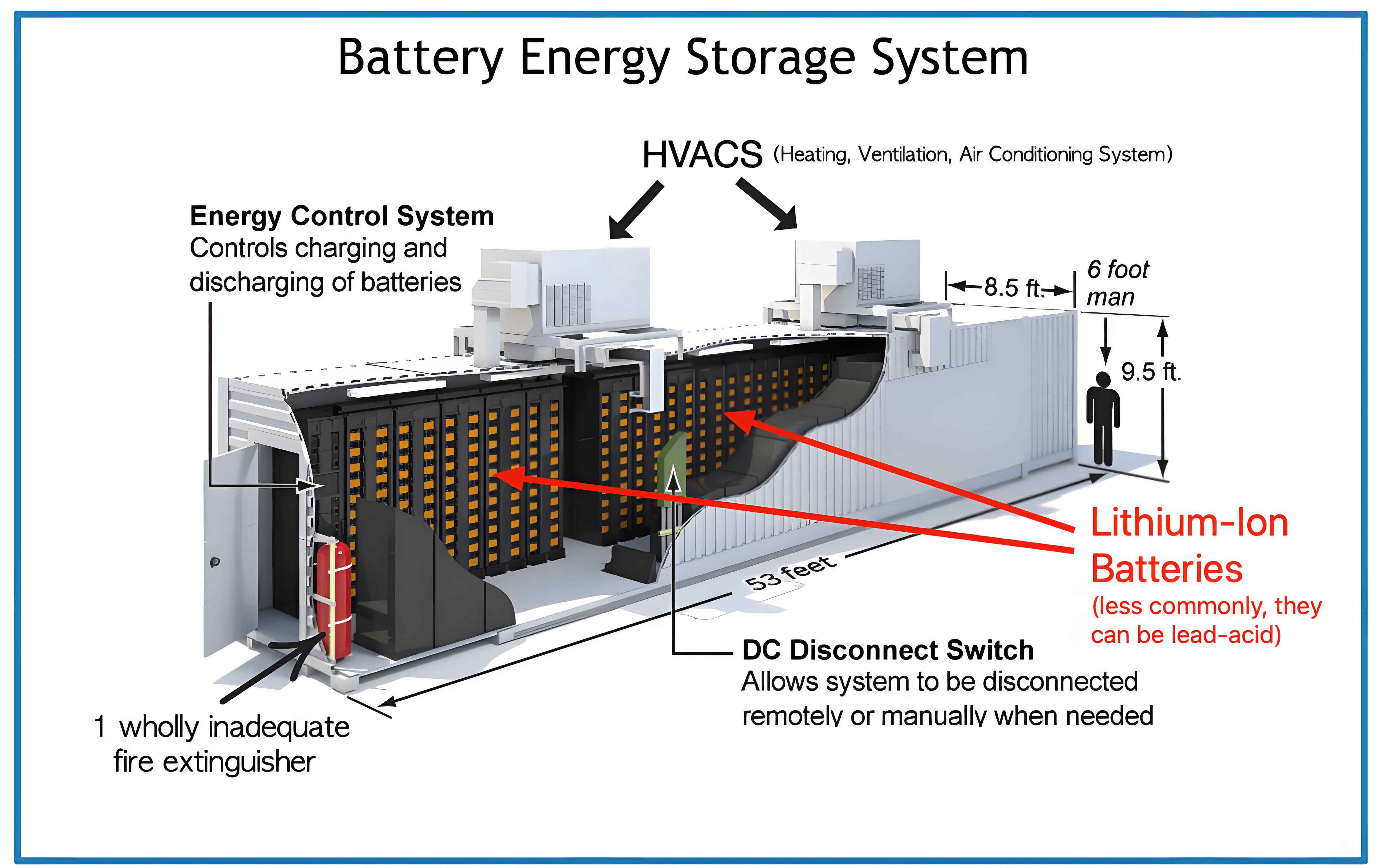
Battery Energy Storage System (energy storage system) has emerged as a pivotal technology to address these challenges, owing to its rapid charge/discharge capability, high energy conversion efficiency, and precise controllability. The energy storage system can perform real-time power compensation to smooth PV output fluctuations and participate in grid auxiliary peak-shaving services by shifting energy across time. However, the relatively high investment cost and limited service life of energy storage system remain critical barriers to widespread deployment. Therefore, it is of paramount importance to develop operation control strategies that not only fulfill technical requirements but also minimize battery degradation, reduce charge/discharge conversion frequency, and prevent state of charge (SOC) excursions.
This study focuses on a PV power station integrated with an energy storage system, investigating control strategies for three application scenarios: PV fluctuation mitigation, grid auxiliary peak-shaving, and multi-scenario collaborative optimization. The main contributions are organized as follows: Section 2 presents the characteristics analysis and modeling of PV systems and battery energy storage systems. Section 3 proposes a secondary power allocation-based control strategy for PV fluctuation smoothing. Section 4 develops a dynamic grouping-based control strategy for grid auxiliary peak-shaving. Section 5 establishes an event-triggered multi-scenario collaborative optimization framework. Section 6 concludes the paper with key findings and future research directions.
2. Modeling of PV Output Characteristics and Battery Energy Storage System
2.1 PV Output Characteristics Modeling
The power output of a PV array can be described by the following engineering model. The (U-I) output characteristic relationship of a PV cell is formulated as:
$$I = I_{SC}\left[1 – C_1 \left(e^{\frac{U}{C_2 U_{OC}}} – 1\right)\right]$$
$$C_1 = \left(1 – \frac{I_m}{I_{SC}}\right) e^{-\frac{U_m}{C_2 U_{OC}}}$$
$$C_2 = \left(\frac{U_m}{U_{OC}} – 1\right) \left[\ln\left(1 – \frac{I_m}{I_{SC}}\right)\right]^{-1}$$
where $U_{OC}$ denotes the open-circuit voltage, $I_{SC}$ the short-circuit current, $U_m$ and $I_m$ represent the voltage and current at the maximum power point, and $C_1$, $C_2$ are correction coefficients. To account for varying irradiance and temperature conditions, the following compensation coefficients are introduced:
$$\Delta I = \alpha \left(\frac{S}{S_{ref}}\right) \Delta t + \left(\frac{S}{S_{ref}} – 1\right)$$
$$\Delta U = \beta \left(t – t_{ref}\right) + b \ln\left(\frac{S}{S_{ref}}\right)$$
where $S$ is the solar irradiance, $S_{ref}$ is the irradiance under standard test conditions, $t$ is the cell temperature, $\alpha$ is the temperature compensation coefficient for current, $\beta$ is the temperature compensation coefficient for voltage, and $b$ is the irradiance compensation coefficient.
2.2 Battery Energy Storage System Modeling
To accurately capture the dynamic characteristics of lithium-ion batteries, the improved PNGV equivalent circuit model is adopted in this work. This model accounts for the triple polarization effects including ohmic polarization, concentration polarization, and electrochemical polarization. The terminal voltage $U_o$ can be expressed as:
$$U_o = U_{oc} – IR_i – U_{ad} – U_{pe} – U_{pc}$$
The state equations governing the polarization capacitances are given by:
$$\begin{bmatrix} \frac{dU_{ad}}{dt} \\ \frac{dU_{pe}}{dt} \\ \frac{dU_{pc}}{dt} \end{bmatrix} = \begin{bmatrix} 0 & 0 & 0 \\ 0 & -\frac{1}{R_{pe}C_{pe}} & 0 \\ 0 & 0 & -\frac{1}{R_{pc}C_{pc}} \end{bmatrix} \begin{bmatrix} U_{ad} \\ U_{pe} \\ U_{pc} \end{bmatrix} + \begin{bmatrix} \frac{1}{C_{ad}} \\ \frac{1}{C_{pe}} \\ \frac{1}{C_{pc}} \end{bmatrix} I$$
where $U_{oc}$ is the open-circuit voltage, $R_i$ is the internal resistance, $R_{pe}$ and $C_{pe}$ are the electrochemical polarization resistance and capacitance, $R_{pc}$ and $C_{pc}$ are the concentration polarization resistance and capacitance, and $C_{ad}$ is the additional capacitance.
The SOC of each battery unit is calculated as:
$$SOC(t) = SOC(t-1) + \frac{\eta P(t) \Delta t}{E_b}$$
where $\eta$ denotes the charge/discharge efficiency, $P(t)$ is the power at time $t$, $\Delta t$ is the control interval, and $E_b$ is the rated energy capacity of the battery unit.
3. Secondary Power Allocation Strategy for PV Fluctuation Smoothing
3.1 PV Grid-connected Power Instruction Acquisition Based on IRCA
The Rain-flow Counting Algorithm (RCA) is a classical data compression technique originally developed for fatigue life calculation. It effectively reduces the fluctuation of raw PV power data while preserving essential trend information. However, excessive data compression may degrade the information content. To balance fluctuation reduction with data retention, the Improved Rain-flow Counting Algorithm (IRCA) is proposed with a compression threshold $E$. The compression condition is given by:
$$v_{g,g+1} > 0 \quad \text{and} \quad |P_y(g+1) – P_y(g+2)| > E \quad \text{and} \quad v_{g+2,g+3} < 0$$
where $v_{g,g+1}$ is the slope of the line connecting $P_y(g)$ and $P_y(g+1)$, and $v_{g+2,g+3}$ is the slope between $P_y(g+2)$ and $P_y(g+3)$. The optimal compression threshold $E$ is determined via the Carnivorous Plant Algorithm (CPA) by minimizing the following fitness function:
$$\min f_1 = \alpha_1 C_R + \alpha_2 \overline{P} + \alpha_3 \Delta P + \alpha_4 B$$
where $C_R$ is the compression ratio, $\overline{P}$ represents the power tracking error between the grid-connected instruction and the raw PV power, $\Delta P$ is the average fluctuation rate of the smoothed power, and $B$ is the number of charge/discharge conversion cycles. The power tracking error and BESS power regulation instruction are computed as:
$$\overline{P} = \frac{1}{t”} \sum_{t=1}^{t”} |P_y(t) – P_b(t)|$$
$$P_{BE}(t) = P_y(t) – P_b(t)$$
where $P_b(t)$ is the grid-connected power instruction obtained by IRCA, $P_y(t)$ is the raw PV power, and $P_{BE}(t)$ is the BESS power regulation instruction (positive for charging, negative for discharging).
The average fluctuation rate over the entire dispatch horizon is:
$$\Delta P = \frac{1}{N_g} \sum_{i=1}^{N_g} \frac{\max\{P(t)\} – \min\{P(t)\}}{P_g} \quad t \in [t_i, t_i + T]$$
where $N_g$ is the number of time slots, $T$ is the duration of each slot, and $P_g$ is the installed PV capacity.
3.2 Battery Group Power Allocation Based on Wavelet Packet Transform
After obtaining the BESS power regulation instruction $P_{BE}$, the Wavelet Packet Transform (WPT) is employed to decompose it into multiple frequency components. Each decomposed component corresponds to a battery group, and the number of battery groups $n$ equals $2^k$, where $k$ is the decomposition layer. The optimal decomposition layer is determined by:
$$k = \arg\min \{k \mid 2^k \geq \omega, \quad \delta \leq \alpha_5 \overline{\delta}\}$$
where $\omega$ is the number of battery units, $\delta$ is the standard deviation of $P_{BE}$, $\overline{\delta}$ is the average standard deviation of the $k$-layer decomposition results, and $\alpha_5$ is the weight coefficient optimized via the relationship between $\alpha_5$ and the average battery degradation rate. For the case study in this work, $\alpha_5 = 0.57$ yields the minimum average battery degradation at $k = 2$, resulting in 4 battery groups.
Based on the decomposition results, the rated power of each battery group is determined by taking the 90th percentile of the absolute power values. The capacities of the four battery groups are configured as 2 MW/4 MWh, 1 MW/2 MWh, 1 MW/2 MWh, and 1 MW/2 MWh, respectively.
3.3 Dynamic Maximum Charge/Discharge Power Updating
To prevent SOC excursions, the maximum charging and discharging power of each battery unit is dynamically updated based on the real-time SOC:
$$P_{cmax,i,t} = \begin{cases} P_{max} & SOC_{i,t} \leq SOC_{max} – \Delta SOC \\ \frac{SOC_{max} – SOC_{i,t}}{T_b} C_b & SOC_{max} – \Delta SOC < SOC_{i,t} < SOC_{max} \end{cases}$$
$$P_{dmax,i,t} = \begin{cases} -P_{max} & SOC_{i,t} \geq SOC_{min} + \Delta SOC \\ -\frac{SOC_{i,t} – SOC_{min}}{T_b} C_b & SOC_{min} < SOC_{i,t} < SOC_{min} + \Delta SOC \end{cases}$$
where $SOC_{max} = 0.9$, $SOC_{min} = 0.1$, $\Delta SOC = \frac{P_{max} T_b}{C_b}$, $T_b$ is the control period, and $C_b$ is the battery unit capacity. This adaptive approach ensures that as the battery approaches its operational limits, the maximum allowable power is gradually reduced, thereby preventing SOC violations and protecting battery health.
3.4 Battery Unit Power Allocation with Repeated Compensation
For battery units in the group responsible for differential power allocation, a two-stage power allocation process is designed. The initial power allocation follows the SOC balancing principle, where the charging function and discharging function are defined as:
$$f_{cd}(SOC_{i,t}) = 0.5 – 0.33 \cdot \arctan(25 \cdot (SOC_{i,t} – 0.5))$$
$$f_{ds}(SOC_{i,t}) = 0.5 + 0.33 \cdot \arctan(25 \cdot (SOC_{i,t} – 0.5))$$
These functions assign higher charging weights to battery units with lower SOC and higher discharging weights to units with higher SOC, thereby promoting SOC equalization within each group. The charging power allocation is computed as:
$$\frac{P_{U,i,t}}{f_{cd}(SOC_{i,t})} = \frac{P_{U,j,t}}{f_{cd}(SOC_{j,t})}, \quad i,j \in N$$
$$\frac{P_{U,i,t}}{f_{ds}(SOC_{i,t})} = \frac{P_{U,j,t}}{f_{ds}(SOC_{j,t})}, \quad i,j \in N$$
After initial allocation, a repeated compensation principle is implemented to ensure full tracking of the power instruction. If a battery unit’s allocated power exceeds its dynamic maximum, the excess power is redistributed among the remaining units until either the group instruction is fully tracked or all units have reached their limits.
3.5 Simulation Results for PV Fluctuation Smoothing
A case study is conducted on a 50 MW PV station integrated with a 5 MW/10 MWh BESS comprising 20 battery units. Table 1 presents a comparison between IRCA and RCA for extracting the grid-connected power instruction:
| Metric | IRCA | RCA |
|---|---|---|
| Compression ratio $C_R$ | 12% | 6% |
| Power tracking error $\overline{P}$ (MW) | 0.121 | 0.188 |
| Average fluctuation rate $\Delta P$ | 0.0122 | 0.0115 |
Table 2 compares the number of charge/discharge conversions across different methods:
| Method | IRCA | WPT | Low-pass Filter | Variational Mode Decomposition |
|---|---|---|---|---|
| Number of conversions (times) | 30 | 118 | 182 | 180 |
The CPA optimization process shows convergence to the optimal compression threshold $E = 3.0$ within 17 iterations with a fitness value of 149. Table 3 compares the performance of different power allocation strategies:
| Metric | Proposed Strategy | Strategy 1 | Strategy 2 | Strategy 3 | Strategy 4 | Strategy 5 |
|---|---|---|---|---|---|---|
| SOC violation count (times) | 0 | 15 | 0 | 0 | 6 | 22 |
| SOC violation duration (min) | 0 | 492 | 0 | 0 | 195 | 726 |
| Tracking accuracy $\beta$ (%) | 100 | 94.8 | 91.3 | 93.1 | 96.6 | 90.1 |
| Average battery degradation $l$ (%) | 0.00519 | 0.00498 | 0.00489 | 0.00496 | 0.00579 | 0.00535 |
| Expected service life (years) | 10.55 | 11.01 | 11.20 | 11.00 | 9.46 | 10.24 |
| Maximum fluctuation rate (%) | 0.0375 | 0.1186 | 0.1143 | 0.0889 | 0.1215 | 0.0955 |
The results demonstrate that the proposed strategy achieves zero SOC violations, 100% tracking accuracy, and the lowest maximum fluctuation rate of 0.0375%, effectively meeting the grid integration standard while minimizing battery degradation. The dynamic maximum power updating and repeated compensation mechanism are crucial for maintaining tracking accuracy and preventing SOC excursions.
4. Dynamic Grouping-based Control Strategy for Grid Auxiliary Peak-shaving
4.1 Improved Golden Eagle Optimizer
The Golden Eagle Optimizer (GEO) mimics the hunting behavior of golden eagles, which involves attack and cruise phases. In each iteration, an eagle chooses between attacking its prey (intensification) and cruising to explore new areas (diversification). The position update equation is:
$$X_i^{m+1} = X_i^m + \Delta X_i^m$$
$$\Delta X_i^m = r_2 p_a \frac{A_i}{\|A_i\|} + r_3 p_c \frac{C_i}{\|C_i\|}$$
where $p_a$ and $p_c$ are the attack and cruise coefficients, $A_i$ is the attack vector defined as $A_i = X_f^* – X_i$ ($X_f^*$ is the best position found so far), and $C_i$ is the cruise vector computed from the normal hyperplane. The original GEO uses linearly varying coefficients, which can lead to insufficient exploitation in early iterations and poor ability to escape local optima in later stages.
To address these limitations, the Improved Golden Eagle Optimizer (IGEO) is proposed with the following modifications:
(1) Bernoulli Chaotic Initialization: The initial population is generated using Bernoulli chaotic mapping:
$$X_{i+1} = \begin{cases} X_i / (1 – \lambda) & X_i \in (0, 1 – \lambda] \\ (X_i – 1 + \lambda) / \lambda & X_i \in (1 – \lambda, 1) \end{cases}$$
where $\lambda = 0.5$. This enhances the diversity of the initial population and prevents premature convergence.
(2) Improved Attack and Cruise Coefficients:
$$p_a^m = \alpha_1 \cdot \frac{2}{1 + e^m} + \alpha_2$$
$$p_c^m = \alpha_3$$
where $\alpha_1 = -0.2$, $\alpha_2 = 50$, and $\alpha_3 = 0.94$. The nonlinear adjustment of $p_a$ enables stronger global exploration in early iterations and enhanced local exploitation in later iterations.
4.2 BESS Peak-shaving Dispatch Model
The peak-shaving dispatch model aims to minimize the grid load peak-valley difference while maximizing the operational benefits of the energy storage system. The objective function is formulated as:
$$\min f_\varphi = \omega_1 \frac{f_1}{f_{1,max}} + \omega_2 \frac{f_2}{f_{2,max}}$$
where $f_1$ represents the grid load peak-valley difference:
$$f_1 = \max(P_{load}(t) + P_{bess}(t)) – \min(P_{load}(t) + P_{bess}(t))$$
and $f_2$ represents the total operational cost of BESS:
$$f_2 = \sum_{t=1}^{96} \left( C_{charge}(t) + C_{loss}(t) – C_{rev}(t) – C_{carbon}(t) \right)$$
where $C_{charge}(t) = c_{el} \cdot P_{bess}(t)$ is the charging cost, $C_{loss}(t) = c_{loss} \cdot P_{bess}(t) \cdot \Delta t$ is the battery degradation cost, $C_{rev}(t) = c_{carbon} \cdot q_{carbon} \cdot Q_{bess}(t)$ is the carbon credit revenue, and $Q_{bess}(t)$ represents the carbon emission reduction achieved by the energy storage system.
The optimization is subject to the following constraints on battery power, SOC, and charge/discharge status:
$$|P_{bi,t}| \leq |P_{bmax}|$$
$$SOC_{min} \leq SOC_{i,t} \leq SOC_{max}$$
$$s_{ci,t} + s_{di,t} \leq 1$$
where $s_{ci,t}$ and $s_{di,t}$ are binary indicators for charging and discharging states, respectively. The penalty function method is used to convert the constrained optimization problem into an unconstrained one:
$$F = f_\varphi + \theta_1 g_1 + \theta_2 g_2 + \theta_3 g_3$$
where $g_1$, $g_2$, and $g_3$ are violation flags for power limits, capacity limits, and charge/discharge status limits (1 if violated, 0 otherwise), and $\theta_i = 10^8$ are penalty coefficients.
4.3 k-means-based Dynamic Grouping and Two-layer Power Allocation
To enhance the SOC balancing capability of the energy storage system, the k-means clustering algorithm is employed to dynamically partition all battery units into three groups based on their real-time SOC values:
- PCG (Priority Charging Group): Battery units with the lowest SOC values that should be charged first.
- RG (Reserve Group): Battery units with intermediate SOC values.
- PDG (Priority Discharging Group): Battery units with the highest SOC values that should be discharged first.
The k-means algorithm minimizes the sum of squared distances between data points and their assigned cluster centroids:
$$J = \sum_{j=1}^{3} \sum_{i \in C_j} \|SOC_i – \mu_j\|^2$$
where $\mu_j$ is the centroid of cluster $C_j$. The grouping process is updated at each dispatch interval based on the current SOC distribution.
The two-layer power allocation strategy is designed as follows:
Upper-layer allocation: When $P_B > 0$ (charging), the response order is PCG → RG → PDG. The allocation among groups is shown in Table 4:
| State | Condition | PCG | RG | PDG |
|---|---|---|---|---|
| Charging ($P_B > 0$) | $P_B \geq P_{max,c} + P_{max,b}$ | $P_{max,c}$ | $P_{max,b}$ | $P_B – P_{max,c} – P_{max,b}$ |
| $P_{max,c} < P_B < P_{max,c} + P_{max,b}$ | $P_{max,c}$ | $P_B – P_{max,c}$ | 0 | |
| $P_B \leq P_{max,c}$ | $P_B$ | 0 | 0 | |
| Discharging ($P_B < 0$) | $P_B \geq P_{max,d} + P_{max,b}$ | $P_B – P_{max,d} – P_{max,b}$ | $P_{max,b}$ | $P_{max,d}$ |
| $P_{max,d} + P_{max,b} < P_B < P_{max,d}$ | 0 | $P_B – P_{max,d}$ | $P_{max,d}$ | |
| $P_B \geq P_{max,d}$ | 0 | 0 | $P_B$ |
Lower-layer allocation: Within each group, the power is distributed among individual battery units based on the SOC balancing functions:
$$P_i(t) = f_{cd}(SOC_i(t-1)) \cdot \frac{P_{group}(t)}{\sum_{j=1}^{N} f_{cd}(SOC_j(t-1))}, \quad \text{for charging}$$
$$P_i(t) = f_{ds}(SOC_i(t-1)) \cdot \frac{P_{group}(t)}{\sum_{j=1}^{N} f_{ds}(SOC_j(t-1))}, \quad \text{for discharging}$$
where $P_{group}(t)$ is the power instruction allocated to the group, and $N$ is the number of battery units within the group.
4.4 Simulation Results for Peak-shaving
A typical summer daily load curve from a regional grid is used for validation. The BESS has a rated power of 7.5 kW and capacity of 35 kWh with 90% charge/discharge efficiency. Table 5 compares the peak-shaving performance and operational costs across different optimization algorithms:
| Algorithm | Peak-valley difference (kW) | Peak-valley difference rate (%) | Operational cost (CNY/h) |
|---|---|---|---|
| Original load | 1393 | 55.03 | / |
| IGEO | 1148 | 47.92 | 3286 |
| GEO | 1188 | 49.60 | 3957 |
| GA | 1221 | 50.99 | 4330 |
| WOA | 1292 | 53.93 | 4562 |
| PSO | 1310 | 54.69 | 4753 |
The IGEO algorithm achieves the lowest peak-valley difference rate of 47.92% and the lowest operational cost, demonstrating superior performance in both technical and economic aspects. Table 6 compares the battery lifespan under different power allocation strategies:
| Strategy | Battery degradation (kWh) | Service life (years) |
|---|---|---|
| Strategy 1: Uniform power allocation | 0.0040 | 4.8 |
| Strategy 2: SOC-based allocation | 0.0036 | 5.3 |
| Strategy 3: Two fixed groups + uniform | 0.0032 | 6.0 |
| Strategy 4: Two fixed groups + SOC-based | 0.0025 | 7.6 |
| Strategy 5: Three fixed groups + uniform | 0.0021 | 9.0 |
| Proposed strategy (k-means + SOC-based) | 0.0019 | 10.0 |
The proposed dynamic grouping strategy extends the BESS service life to 10 years, a 108% improvement over Strategy 1. The tracking deviation of the BESS remains within 12 kW, and the actual peak-valley difference rate after BESS response is 48.04%. The SOC standard deviation across groups decreases from 0.0847 (before response) to 0.076 (after response), demonstrating improved SOC balance and enhanced dispatch potential.
5. Event-triggered Multi-scenario Collaborative Optimization
5.1 Day-ahead and Intraday Optimization Framework
To enable the energy storage system to participate in both PV fluctuation smoothing and grid auxiliary peak-shaving, a “day-ahead + intraday” two-stage dispatch framework is designed. The day-ahead optimization layer determines the reserved power for PV smoothing and the optimal peak-shaving dispatch plan. The reserved power is estimated based on PV forecast characteristics:
$$P_{s.up} = \begin{cases} 2P_{s.up}^{max} \frac{P_{pvq}}{P_{max}} & P_{pvq} \leq 0.5P_{max} \\ 2P_{s.up}^{max} \left(1 – \frac{P_{pvq}}{P_{max}}\right) & P_{pvq} > 0.5P_{max} \end{cases}$$
where $P_{s.up}^{max}$ is the maximum reserved power (set to 10% of installed capacity), $P_{pvq}$ is the day-ahead PV forecast power, and $P_{max}$ is the installed PV capacity. The remaining power is available for peak-shaving market participation:
$$\max f_D = \sum_{i=1}^{N_D} d_e(i) \cdot (P_{edis}(i) – P_{ech}(i)) \cdot \Delta t$$
where $d_e(i)$ is the real-time energy market price, $P_{edis}(i)$ and $P_{ech}(i)$ are the discharge and charge power in the energy market, respectively.
5.2 PV Fluctuation Smoothing Strategy Based on SOC
In the intraday stage, an event-triggered mechanism dynamically coordinates the dual functions. The fluctuation suppression strategy based on SOC variation is formulated as:
(1) No operation zone: When SOC reaches its limit, charge (when $SOC \geq 0.8$) or discharge (when $SOC \leq 0.2$) is prohibited.
(2) Suppress only threshold-exceeding fluctuations: When the current SOC deviation from the expected value would increase:
$$P_{sch} = \max(0, P_{pv} – P_{pvlim}^{up}) \quad \text{if } SOC \leq 0.8 \text{ and } P_{pv} > P_{pvlim}^{up}$$
$$P_{sdis} = \max(0, P_{pvlim}^{down} – P_{pv}) \quad \text{if } SOC \geq 0.2 \text{ and } P_{pv} < P_{pvlim}^{down}$$
(3) Full compensation mode: When the BESS regulation reduces the SOC deviation:
$$P_{sch} = P_{pv} – P_{pvrq} \quad \text{if } SOC \leq SOC_e \text{ and } P_{pv} < P_{pvrq}$$
where $P_{pvrq}$ is the day-ahead PV forecast power, and $SOC_e$ is the expected SOC.
5.3 Event-triggered Dynamic Priority Control
The event-triggered control mechanism is designed to dynamically switch between fluctuation smoothing and peak-shaving modes:
(1) Event threshold:
$$\Delta P(t) = |P_{pv}^{actual}(t) – P_b(t)| > \delta_{th}$$
where $\delta_{th}$ is the fluctuation threshold set to 5% of the installed PV capacity.
(2) Priority logic: If $\Delta P(t) \geq \delta_{th}$, the system enters “fluctuation smoothing priority” mode, temporarily reducing the peak-shaving power to reserve capacity. If $\Delta P(t) < \delta_{th}$, the system maintains “peak-shaving priority” mode, executing the day-ahead dispatch plan.
(3) Transition mechanism: After the fluctuation event ends (consecutive 3 control periods with $\Delta P(t) < 0.5\delta_{th}$), the system smoothly transitions back to peak-shaving mode using an exponential ramp:
$$P_{peak}^{rec}(t) = P_{peak}^{plan} \cdot \left(1 – e^{-t/\tau}\right)$$
where $\tau = 15$ min is the transition time constant, preventing sudden power changes.
The power coupling constraint is expressed as:
$$P_{sm}(t) + P_{peak}(t) \leq P_{BESS}^{max}$$
5.4 Multi-objective Collaborative Optimization Model
To quantify the trade-off among fluctuation smoothing effectiveness, peak-shaving revenue, and battery degradation, a multi-objective optimization model is formulated:
$$\max f_1 = \sum_{i=1}^{N_D} d_e(i) \cdot (P_{edis}(i) – P_{ech}(i)) \cdot \Delta t$$
$$\min f_2 = \sum_{k=1}^{M} x_1(k)^2 + \alpha \cdot (SOC_s(k) – SOC_e(k))^2$$
where $x_1(k)$ is the deviation between PV-plus-storage output and the day-ahead PV forecast, $M$ is the number of control intervals, and $\alpha$ is the penalty coefficient.
To solve this multi-objective problem, the Multi-Objective Improved Golden Eagle Optimizer (MO-IGEO) is developed by integrating non-dominated sorting and crowding distance computation into the IGEO framework. The non-dominated sorting partitions solutions into Pareto fronts, while the crowding distance ensures solution diversity:
$$CrowdingDistance(i) = \sum_{m=1}^{M} \frac{f_m(i+1) – f_m(i-1)}{f_m^{max} – f_m^{min}}$$
5.5 Simulation Results for Multi-scenario Optimization
Based on a 50 MW PV station and regional grid peak-shaving requirements, three scenarios are compared: Scenario 1 (smoothing only), Scenario 2 (peak-shaving only), and Scenario 3 (collaborative optimization). Table 7 presents the performance comparison:
| Metric | Scenario 1 (Smoothing only) | Scenario 2 (Peak-shaving only) | Scenario 3 (Collaborative) |
|---|---|---|---|
| Post-smoothing fluctuation rate (%) | 0.382 | / | 0.891 |
| Peak-valley difference rate (%) | / | 47.92 | 47.89 |
| Peak-shaving revenue (CNY/day) | 0 | 7,886.4 | 8,264.7 |
| Degradation cost (CNY/day) | 1,532.1 | 2,187.5 | 1,845.3 |
| Net revenue (CNY/day) | -1,532.1 | 5,698.9 | 6,419.4 |
| SOC balance (standard deviation) | 0.072 | 0.084 | 0.069 |
| Degradation rate (×10⁻⁴ %/h) | 21.0 | 19.0 | 18.0 |
The collaborative optimization scenario achieves the best overall performance: the highest net revenue, lowest degradation rate, and best SOC balance. The event-triggered mechanism effectively reduces the grid-connected power standard deviation from 1.82 MW to 0.64 MW during fluctuation events, while the peak-shaving revenue loss is limited to only 2.3% during the transition period.
Sensitivity analyses reveal that the collaborative strategy maintains robust performance under uncertain electricity prices, with the revenue variation rate at ±8.7% under a ±30% price fluctuation range (compared to ±12.1% for the single peak-shaving strategy). When BESS capacity increases from 10 MW to 15 MW, the collaborative strategy achieves a 21.3% net revenue improvement (compared to 14.8% for peak-shaving only).
Table 8 compares the algorithm performance among MO-IGEO, NSGA-II, and MOPSO:
| Metric | MO-IGEO | NSGA-II | MOPSO |
|---|---|---|---|
| Convergence generation | 62 | 85 | 78 |
| Hypervolume (HV) | 0.872 | 0.785 | 0.721 |
| Best solution (BS) | 1.25 | 1.32 | 1.40 |
| RMSE | 0.012 | 0.015 | 0.018 |
| Computational time (s) | 18.3 | 24.7 | 21.5 |
MO-IGEO achieves 27% faster convergence than NSGA-II and an 11.1% improvement in HV, demonstrating superior multi-objective optimization capability. The event-triggered mechanism, with the two-level thresholds (5% and 10% of rated power), successfully balances rapid response to severe fluctuations (full smoothing priority) with minimal disruption to peak-shaving economics (proportional power reduction in warning mode).
6. Conclusion and Future Work
This dissertation investigates operation control strategies for battery energy storage systems (energy storage system) applied in multiple scenarios, including PV fluctuation smoothing, grid auxiliary peak-shaving, and coordinated multi-scenario optimization. The main conclusions are summarized as follows:
(1) Secondary power allocation-based PV fluctuation smoothing strategy: The IRCA-based approach, optimized by CPA, successfully reduces the charge/discharge conversion frequency by 75% compared to conventional filtering methods while satisfying grid integration standards. The WPT-based dynamic grouping and two-stage power allocation strategy prevents SOC excursions, achieves accurate tracking of power instructions, and limits average battery degradation to 0.0519%, thereby significantly extending the safe operation lifetime of the energy storage system.
(2) Dynamic grouping-based peak-shaving strategy: The IGEO algorithm demonstrates superior optimization performance over GEO, PSO, WOA, and GA in terms of solution quality and convergence speed. The optimization of peak-shaving dispatch reduces the peak-valley difference rate from 55.03% to 48.04% and reduces BESS operational costs. The k-means dynamic grouping method effectively improves SOC balance (standard deviation reduced from 0.0847 to 0.076), extends service life to 10 years (doubling the baseline of 4.8 years), and enhances the dispatch potential of the energy storage system.
(3) Event-triggered multi-scenario collaborative optimization: The “day-ahead + intraday” dispatch framework with dynamic event triggering enables the energy storage system to seamlessly coordinate between PV fluctuation smoothing and grid peak-shaving, effectively resolving the conflicts in time scales, power requirements, and objective functions. The MO-IGEO algorithm demonstrates strong robustness to price uncertainty and capacity variations. The collaborative strategy achieves the highest net revenue among all scenarios, reduced degradation rates by 5.3% compared to single-function scenarios, improved SOC balance, and reduced grid-connected power standard deviation from 1.82 MW to 0.64 MW during fluctuation events. The peak-valley difference rate further decreases to 47.89%.
Future research directions may include: (1) incorporating deep reinforcement learning to enhance the adaptive capability of the proposed control strategies under extreme weather conditions and complex market mechanisms; (2) extending the multi-scenario framework to integrate additional grid services such as frequency regulation and reserve capacity; and (3) investigating the optimal sizing of energy storage system under multi-scenario collaborative operations to further improve economic viability.