
1. Introduction
With the acceleration of energy transformation and digitalization, the installed capacity of renewable energy in power systems has been increasing year by year. The intermittent, random, and volatile characteristics of renewable energy generation have brought severe challenges to the safe and stable operation of power systems. The role of energy storage technology in power systems has become increasingly important, and power energy storage facilities have become indispensable components in grid operation. Their operational flexibility is of positive significance for ensuring grid security and promoting the consumption of renewable energy sources such as wind and photovoltaic power.
By the end of 2023, the cumulative installed capacity of global power energy storage projects had reached 289.2 GW, with an annual growth rate of 21.9%. The energy storage industry in China has also developed rapidly, with the cumulative installed capacity of energy storage projects reaching 86.5 GW by the end of 2023. The proportion of pumped hydro storage installations has been decreasing year by year, while the proportion of lithium battery installations has been increasing annually. In recent years, electrochemical energy storage has gained increasing market share due to its advantages of flexible usage and fast response speed. Compared to traditional energy storage methods, electrochemical energy storage offers higher energy density and higher energy conversion efficiency.
The energy storage system, as an efficient energy storage and release solution, plays a crucial role in stabilizing power system power fluctuations, improving transient response characteristics, and supporting safe and stable power system operation. Accurate transient models and parameters are key to studying the support capability of the energy storage system. The energy storage system can effectively overcome the uncertainty caused by renewable energy changes through flexible charging and discharging operations. Furthermore, to fully exploit the regulation potential of the energy storage system, it is necessary to reasonably configure the control parameters of the energy storage system to adapt to the regulation requirements of renewable energy grid-connected operation. Therefore, studying the parameter identification and control optimization methods of the energy storage system is of great significance, providing model foundations and data support for practical engineering applications.
2. Literature Review
2.1 Research Status of Energy Storage System Modeling
The modeling research of the energy storage system can be mainly divided into electromagnetic transient models and electromechanical transient models based on simulation step size. Electromagnetic transient models are mainly used to study the behavior of the energy storage system during transient electromagnetic processes. Electromechanical transient simulation models involve the interaction between mechanical and electrical systems, mainly used to study the response of the energy storage system during mechanical rotation and electrical processes.
With the continuous increase of clean energy installed capacity, the grid connection of volatile and intermittent renewable energy has brought many challenges to the new power system. Energy storage modeling has gradually shifted from computationally complex electromagnetic transient models to electromechanical transient models that observe the system dynamic response process. In previous research on transient modeling of energy storage systems, some simplified models ignored the representation of State of Charge (SOC), which no longer meets the requirements for electromechanical transient modeling of energy storage systems. To accurately reflect the transient characteristics of the energy storage system, it is necessary to study the energy storage battery and converter to establish accurate models.
2.2 Research Status of Energy Storage System Parameter Identification
Controller parameters directly affect the dynamic response characteristics of the energy storage system, and conducting parameter identification research is of significant practical engineering importance. Inaccurate parameters may lead to system instability or performance degradation during transient events. Through parameter identification research, parameter errors can be reduced, improving the understanding and prediction capability of the energy storage system’s behavior.
Current research on parameter identification of the energy storage system mainly focuses on two aspects: battery parameters and converter parameters. For battery parameter identification, least squares methods and equivalent circuit models are commonly used. For converter parameter identification, most methods identify parameters based on small-signal models, which may not accurately describe the transient characteristics of the energy storage system in practical applications. Additionally, parameter sensitivity analysis of the energy storage system controller has rarely been addressed in existing literature.
2.3 Research Status of Energy Storage System Control Optimization
In the field of power system frequency stability, researchers have proposed various adaptive power control methods and inertial simulation strategies. In the field of voltage stability, joint voltage regulation strategies combining energy storage with capacitors have been studied. In the field of power angle stability, wind-storage joint control methods and regional coordination strategies have been proposed.
However, existing research on transient stability problems has mostly focused on control strategies and transient potential energy indicators, with fewer studies on parameter optimization configuration of energy storage controllers. Therefore, there is an urgent need to conduct research on parameter optimization configuration for power system transient stability to fully exploit the regulation potential of the energy storage system.
3. Electromechanical Transient Modeling of the Energy Storage System
3.1 Model Structure
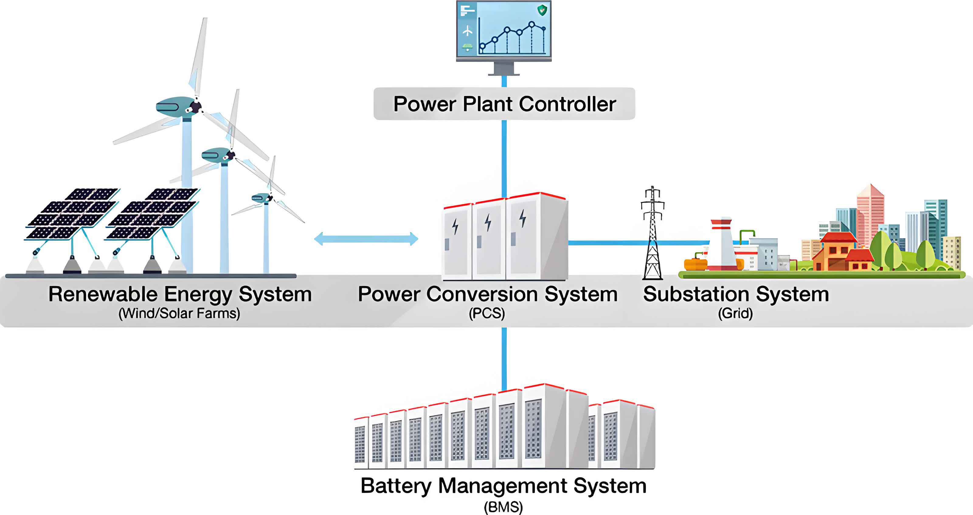
The energy storage system generally consists of three parts: the energy storage battery, the monitoring system, and the power conversion system (PCS). In DIgSILENT-PowerFactory simulation software, PWM converters connected to controlled voltage sources are typically used to represent the energy storage system. However, for electromechanical transient simulation, static generators can be considered as current sources, with active and reactive reference currents as control inputs. Therefore, the energy storage battery model and converter model can be encapsulated into a static generator, allowing the static generator to serve as the grid interface.
The static generator model implements PQ control through the active current ip and reactive current iq output by the converter model, delivering active and reactive power to the grid. The following equations describe this relationship:
$$P = u_d i_d + u_q i_q$$
$$Q = u_q i_d – u_d i_q$$
For symmetric three-phase voltages, the equations can be simplified to:
$$P = u_d i_d$$
$$Q = -u_d i_q$$
3.2 Converter Electromechanical Transient Model
The inner-loop control of the converter generally employs current control, generating dq-axis components of active and reactive currents to control the magnitude and direction of current. After simplification, the current-loop closed-loop transfer function on the d-axis can be expressed as:
$$G_{cp}(s) = \frac{i_d(s)}{i_{dref}(s)} = \frac{1}{Ls + R + \frac{k_{pp}s + k_{ip}}{s}}$$
With appropriate parameter selection, this can be further simplified to a first-order inertia element:
$$G_{cp}(s) = \frac{i_d(s)}{i_{dref}(s)} = \frac{1}{T_{ip}s + 1}$$
$$G_{cq}(s) = \frac{i_q(s)}{i_{qref}(s)} = \frac{1}{T_{iq}s + 1}$$
where Tip and Tiq are the time constants of the d and q-axis current loops respectively.
3.3 Energy Storage Battery Electromechanical Transient Model
Considering the typical discharge characteristics of lead-acid batteries, when the SOC is between 0.2 p.u. and 0.8 p.u., the voltage and internal resistance changes are relatively small. Therefore, within this interval, the time-varying characteristics of the battery can be ignored. The SOC value of the energy storage system can be calculated as:
$$SOC = SOC_{ini} – \frac{1}{3600 \cdot S_{BESS}} \int_{0}^{t} P_{BESS} \, dt$$
where SOCini is the initial state of charge, PBESS is the active power output, and SBESS is the apparent power of the energy storage system.
3.4 Controller Design
The frequency controller adopts droop control, where the droop coefficient Kdroop determines the relationship between frequency deviation and power output:
$$dp_{ref} = K_{droop}(f_{ref} – f_e)$$
Dead zones are set to avoid frequent operation of the frequency controller. The active power control section adopts active power deviation control, where the active power deviation dp is processed through a PI controller to generate the d-axis current reference signal:
$$dp = p_{ref} + dp_{ref} – P_e$$
$$i_{d\_ref\_in} = (K_p + \frac{1}{sT_p}) \cdot dp$$
The reactive power control section adopts constant voltage control, where the voltage deviation dv is processed through a PI controller to generate the q-axis current reference signal:
$$i_{q\_ref\_in} = (K_q + \frac{1}{sT_q}) \cdot dv$$
The charging/discharging controller manages the battery operation based on SOC limits and implements current limiting strategies. For the energy storage battery, when the SOC exceeds the established range, the battery stops charging/discharging operations. The boundary values of SOC are 0.2 p.u. and 0.8 p.u. For the converter, the current limiting strategy is set to prioritize active power. To enhance the fault ride-through capability of the energy storage system, when the bus voltage drops by more than 0.1 p.u., the dq-axis current values are exchanged to prioritize reactive power.
3.5 Simulation Analysis
A single-machine dual-load system was built in DIgSILENT to verify the effectiveness of the established model. The system parameters are summarized in the following table:
| Component | Active Power (MW) | Reactive Power (Mvar) |
|---|---|---|
| Generator G1 | 50 | 20 |
| Load A | 10 | 2 |
| Load B | 50 | 10 |
The energy storage model parameters are listed below:
| Parameter | Kp | Tp | Tip | Kq | Tq | Tiq | Kdroop |
|---|---|---|---|---|---|---|---|
| Value | 1 | 0.1 | 0.01 | 1 | 0.1 | 0.01 | 0.04 |
Scenario 1: Single-phase grounding fault. At t=0.5s, an a-phase grounding fault occurred at bus 2, eliminated at t=0.63s. The simulation results showed that the energy storage system immediately provided active and reactive power support upon fault occurrence, with output curves peaking at the moment of fault clearance and gradually decreasing to zero during system stabilization.
The comparison of system response with and without the energy storage system showed that the frequency recovery speed at bus 1 was significantly improved, with the descent time after the frequency nadir reduced from 8.83s to 3.07s. Under the constant voltage control strategy, the voltage nadir at bus 1 improved from 0.395 p.u. to 0.420 p.u., with the voltage recovery speed also noticeably enhanced over the case without the energy storage system.
Scenario 2: Load step disturbance. At t=0.1s, load B experienced a step change, with active and reactive power increasing by 60%, restored at t=1.1s. Different energy storage capacity configurations (10 MVA, 30 MVA, 70 MVA) were compared. With increasing energy storage capacity, the generator speed, bus frequency, and voltage all improved. The SOC curves correctly reflected the charging/discharging changes of the energy storage system, and the convergence speed of the SOC curves gradually increased with higher active power output.
4. Parameter Identification of Energy Storage System Controller
4.1 Parameter Identifiability Analysis
Parameter sensitivity refers to the degree of response of the system to parameter changes. Trajectory sensitivity examines the system’s response over a period of time, which needs to account for the system’s dynamic behavior. The trajectory sensitivity of the output variables to the parameters is defined as:
$$S_{\theta_j}^y(t) = \lim_{\Delta\theta_j \to 0} \frac{y(t, \theta_1, …, \theta_j + \Delta\theta_j, …, \theta_m) – y(t, \theta_1, …, \theta_j, …, \theta_m)}{\Delta\theta_j}$$
Using a single-machine infinite bus system containing the energy storage system as the test system, trajectory sensitivity analysis was performed under two disturbance scenarios: three-phase short-circuit fault and P/U reference step disturbance. The selected observation quantities included the active power, reactive power, and voltage of the energy storage system.
The key findings from the trajectory sensitivity analysis are summarized below:
| Observation Quantity | d-axis Parameters | q-axis Parameters |
|---|---|---|
| Active Power P | High sensitivity | Low sensitivity |
| Reactive Power Q | Low sensitivity | High sensitivity |
| Voltage U | Very low sensitivity | Very low sensitivity |
Under both disturbance scenarios, the trajectory sensitivity patterns were similar. The voltage observation quantity exhibited significantly lower overall sensitivity compared to active and reactive power, rendering voltage unsuitable as an identification observation. Selecting active power as the observation quantity for d-axis parameters and reactive power for q-axis parameters was deemed appropriate for effective identification.
4.2 Parameter Identification Scheme
DIgSILENT provides built-in parameter identification functionality. The identification process compares simulated data with measured data to minimize the objective function. The default objective function is the sum of squares of differences between measured and simulated data:
$$F_p = \sum_{i=1}^{n} \omega_i (M_i – S_i)^p$$
where Mi is the measured data, Si is the simulated data, ωi is the weighting factor, and p is the exponential value (default 2).
Based on the sensitivity analysis results, the objective function for the parameter identification was formulated as:
$$F_p = \sum_{i=1}^{n} \omega_1 (M_{i1} – S_{i1})^2 + \sum_{i=1}^{n} \omega_2 (M_{i2} – S_{i2})^2$$
where Mi1 and Si1 represent the measured and simulated active power data, Mi2 and Si2 represent the measured and simulated reactive power data, and ω1 and ω2 are the corresponding weighting factors.
The implementation of parameter identification in DIgSILENT involves four main steps: (1) setting disturbances; (2) building the parameter identification module; (3) designing the identification algorithm; and (4) importing measured data. The identification test system used the same system configuration as the parameter sensitivity analysis, with three-phase short-circuit fault and step disturbance as test scenarios.
4.3 Identification Results Analysis
4.3.1 Short-circuit Fault Scenario
Under the three-phase short-circuit fault scenario, the identification results are presented below:
| Parameter | True Value | Identified Value | Error |
|---|---|---|---|
| Kp | 3 | 2.8434 | -5.22% |
| Tp | 0.02 | 0.0196 | -2.00% |
| Tip | 0.05 | 0.0473 | -5.40% |
| Kq | 3 | 3.0124 | 0.41% |
| Tq | 0.02 | 0.0140 | -30.00% |
| Tiq | 0.05 | 0.0498 | -0.40% |
The identification accuracy ranking was Kq, Tiq, Tp, Kp, Tip, Tq. The q-axis parameters, except for Tq, achieved identification errors within 0.5%. The d-axis parameters showed overall good identification performance with errors around 5%. The Tq identification result was poor, with an error reaching -30%, consistent with the parameter sensitivity analysis where Tq exhibited very low sensitivity. The identified curves of active power, reactive power, voltage, and current showed excellent agreement with the measured curves.
4.3.2 Step Disturbance Scenario
Under the step disturbance scenario, the identification results are summarized below:
| Parameter | True Value | Identified Value | Error |
|---|---|---|---|
| Kp | 3 | 3.0133 | 0.44% |
| Tp | 0.02 | 0.0199 | -0.50% |
| Tip | 0.05 | 0.0505 | 1.00% |
| Kq | 3 | 3.1434 | 4.78% |
| Tq | 0.02 | 0.0124 | -38.00% |
| Tiq | 0.05 | 0.0479 | -4.20% |
Under the step disturbance, the d-axis parameters achieved high identification accuracy, with Kp and Tp errors within 1%. The identification results were consistent with the trajectory sensitivity analysis. The energy storage dynamic response curves fitted well with the measured curves. Combining the identification results under both scenarios, the short-circuit fault produced better q-axis parameter identification, while the step disturbance produced better d-axis parameter identification. For applications requiring high parameter accuracy, different disturbance modes can be selected for different controller parameters.
5. Parameter Optimization for Power System Transient Stability
5.1 Transient Stability Analysis
Power system stability assessment includes frequency stability, voltage stability, and power angle stability. For transient stability, the main focus is on the power angle oscillation of synchronous generators. The criterion for transient stability is that after a major disturbance, the relative power angles between generators increase and return to stable equilibrium after the first or second oscillation period, with gradually decaying oscillations until the system voltages recover.
To analyze the impact of the energy storage system on power angle stability, a single-machine infinite bus system with the energy storage system was used. Through linearization of the system stability operating point, the electromagnetic torque increment of the generator and the active power deviation of the energy storage system can be expressed as:
$$\Delta M_e = k_{c1}\Delta\delta_1 + k_{c2}\Delta P_S$$
Simplifying the energy storage system as a first-order inertia element, the active power output of the energy storage system can be expressed as:
$$\Delta P_S = \frac{k_{e1}\Delta P_G}{1 + Ts}$$
Through derivation, the synchronization torque coefficient KS and damping torque coefficient KD can be obtained:
$$K_S = k_{c1} + \frac{k_{c2}k_{e1}k_{d1}}{1 – k_{e1}k_{d2}}$$
$$K_D = \frac{k_{c2}k_{e1}k_{d1}T}{1 – k_{e1}k_{d2}}$$
From these expressions, the active power deviation coefficient ke1 of the energy storage system can affect both the synchronization torque and damping torque of the generator. Therefore, with reasonable configuration of the energy storage system controller parameters, the system transient stability can be effectively improved.
5.2 DIgSILENT-Python Co-simulation Framework
The built-in optimization modules in DIgSILENT can only optimize components with measurement functions. Since generator power angles and damping parameters lack measurement facilities, these data cannot be directly obtained. To address this limitation, a DIgSILENT-Python co-simulation framework was developed.
The framework integrates four key functions: automatic simulation execution in DIgSILENT; result file export and data reading in Python; parameter optimization computation in Python; and automatic parameter modification back to DIgSILENT. The interface implementation involves several crucial API calls including GetApplication, GetFromStudyCase, GetCalcRelevantObjects, GetAttribute, and SetAttribute functions.
The co-simulation framework operates efficiently without frequent file I/O operations, as Python can directly access and modify internal parameters of DIgSILENT. The validation tests confirmed that the framework successfully achieved data acquisition, parameter modification, and automatic simulation control.
5.3 Parameter Optimization Method
The optimization objective focuses on minimizing the sum of squared errors (SSE) of generator power angles, with a constraint on the voltage SSE of the central node to prevent voltage overshoot:
$$F_{G\_SSE} = \min \sum_{m=1}^{n} \sum_{i=1}^{k} (t_{mi} – a)^2$$
subject to:
$$\sum_{j=1}^{x} (l_{no\_j} – b)^2 – \sum_{j=1}^{x} (l_{with\_j} – b)^2 \geq 0$$
where tmi is the transient power angle of the m-th generator at time i, a is the steady-state power angle, lno_j and lwith_j are the transient voltages before and after the energy storage system integration, and b is the steady-state voltage.
The Particle Swarm Optimization (PSO) algorithm was selected for the optimization. The update equations for velocity and position are:
$$v_i(t+1) = \omega v_i(t) + c_1 r_1 (p_{best,i} – x_i(t)) + c_2 r_2 (g_{best} – x_i(t))$$
$$x_i(t+1) = x_i(t) + v_i(t+1)$$
The PSO algorithm parameters were configured as follows:
| Parameter | Value | Parameter | Value |
|---|---|---|---|
| Population size P | 20 | Iterations I | 200 |
| C1 | 1 | C2 | 1.4 |
| Dim D | 7 | Inertia ω | 0.7 |
5.4 Optimization Results
An IEEE 9-bus system incorporating the energy storage system was used as the test case. A three-phase short-circuit fault was applied to line 5-7 at t=0.5s, cleared at t=0.62s, with a total simulation time of 10s. The controller parameters before and after optimization are:
| Parameter | Kp | Tp | Tip | Kq | Tq | Tiq | Kdroop | Objective |
|---|---|---|---|---|---|---|---|---|
| Measured | 2 | 0.01 | 0.01 | 2 | 0.01 | 0.01 | 0.004 | 348.591 |
| Optimized | 4.824 | 0.020 | 0.005 | 5.012 | 0.014 | 0.005 | 0.011 | 323.442 |
| Range | [1,20] | [0.0001,1) | [0.0001,1) | [1,20] | [0.0001,1) | [0.0001,1) | [0.002,0.04] | — |
The optimization results show that the objective function value decreased from 348.591 to 323.442, representing a 7.21% improvement. The first swing angle of generator G2 decreased from 86.928 degrees (without the energy storage system) to 85.825 degrees (with measured parameters) and further to 85.180 degrees (with optimized parameters). Similarly, for generator G3, the first swing angle decreased from 67.272 degrees to 65.079 degrees, then to 64.235 degrees.
The voltage SSE indicators for the central node were calculated as follows:
| Scenario | Without Energy Storage System | With Measured Parameters | With Optimized Parameters |
|---|---|---|---|
| Voltage SSE | 1.273 | 1.259 | 1.237 |
To verify the adaptability of the optimized parameters under different disturbance scenarios, two additional cases were examined:
Case 1: Load step disturbance. At t=0.5s, load C decreased by 80%, restored at t=1.5s. The SSE indicators are summarized below:
| SSE Indicator | Without Energy Storage System | With Measured Parameters | With Optimized Parameters |
|---|---|---|---|
| G2 | 82.728 | 72.512 | 70.098 |
| G3 | 76.738 | 68.619 | 66.876 |
| Bus 4 | 0.275 | 0.166 | 0.145 |
Case 2: Single-phase grounding fault. At t=0.5s, an a-phase grounding fault occurred at bus 9, cleared after 0.1s. The SSE indicators are:
| SSE Indicator | Without Energy Storage System | With Measured Parameters | With Optimized Parameters |
|---|---|---|---|
| G2 | 155.396 | 134.823 | 128.278 |
| G3 | 142.427 | 129.703 | 125.758 |
| Bus 4 | 1.172 | 1.137 | 1.122 |
The experimental results demonstrate that the optimized parameters effectively reduce the first swing angle of generators and smooth power angle oscillations across multiple fault scenarios. The energy storage system with optimized parameters consistently outperformed both the no-storage configuration and the configuration with measured parameters in improving system transient stability and accelerating central node voltage recovery. The optimized parameters exhibited good adaptability to various disturbance types, ensuring safe and stable power system operation.
6. Conclusion
This research has made the following contributions to the field of energy storage system parameter identification and control optimization:
(1) Electromechanical transient modeling of the energy storage system. A simplified energy storage system electromechanical transient model was established that ignores high-frequency electronic components. The model incorporates the energy storage battery characteristics, converter dynamics represented by first-order inertia elements, and comprehensive controller designs including frequency droop control, PV active power control, constant voltage reactive power control, and charging/discharging management with current limiting strategies. Simulation results confirmed that the model effectively reflects the transient response characteristics of the energy storage system and provides excellent dynamic regulation capability for the power grid.
(2) Parameter identification strategy. A parameter identification strategy based on the transient trajectory of the energy storage system was proposed. Through trajectory sensitivity analysis, it was determined that active power is suitable for observing d-axis parameters while reactive power is suitable for observing q-axis parameters. The identification framework and strategy were validated on the test system under both circuit fault and step disturbance scenarios. The results demonstrated that the identification errors for the energy storage system controller parameters were generally within 5% for most parameters and could reach as low as 0.5% for highly sensitive parameters. The identification results exhibited a positive correlation with parameter trajectory sensitivity.
(3) Parameter optimization method based on DIgSILENT-Python co-simulation. A joint simulation framework was developed to enable automated data exchange between DIgSILENT and Python, overcoming the limitation that DIgSILENT can only optimize targets with measurement functions. Combined with the PSO algorithm, the framework effectively optimized the energy storage system controller parameters. The optimized parameters reduced the generator first swing angle, smoothed power angle oscillations, and improved central node voltage recovery. The optimization effect was verified across multiple fault scenarios including three-phase short-circuit faults, load step disturbances, and single-phase grounding faults.
Future research directions include incorporating high- and low-voltage ride-through control strategies for enhanced fault ride-through capability of the energy storage system, expanding the parameter identification approach to cover additional disturbance scenarios encountered in practical grid-connected operation, and investigating improved optimization algorithms to further enhance the accuracy and efficiency of energy storage system parameter identification and optimization.