
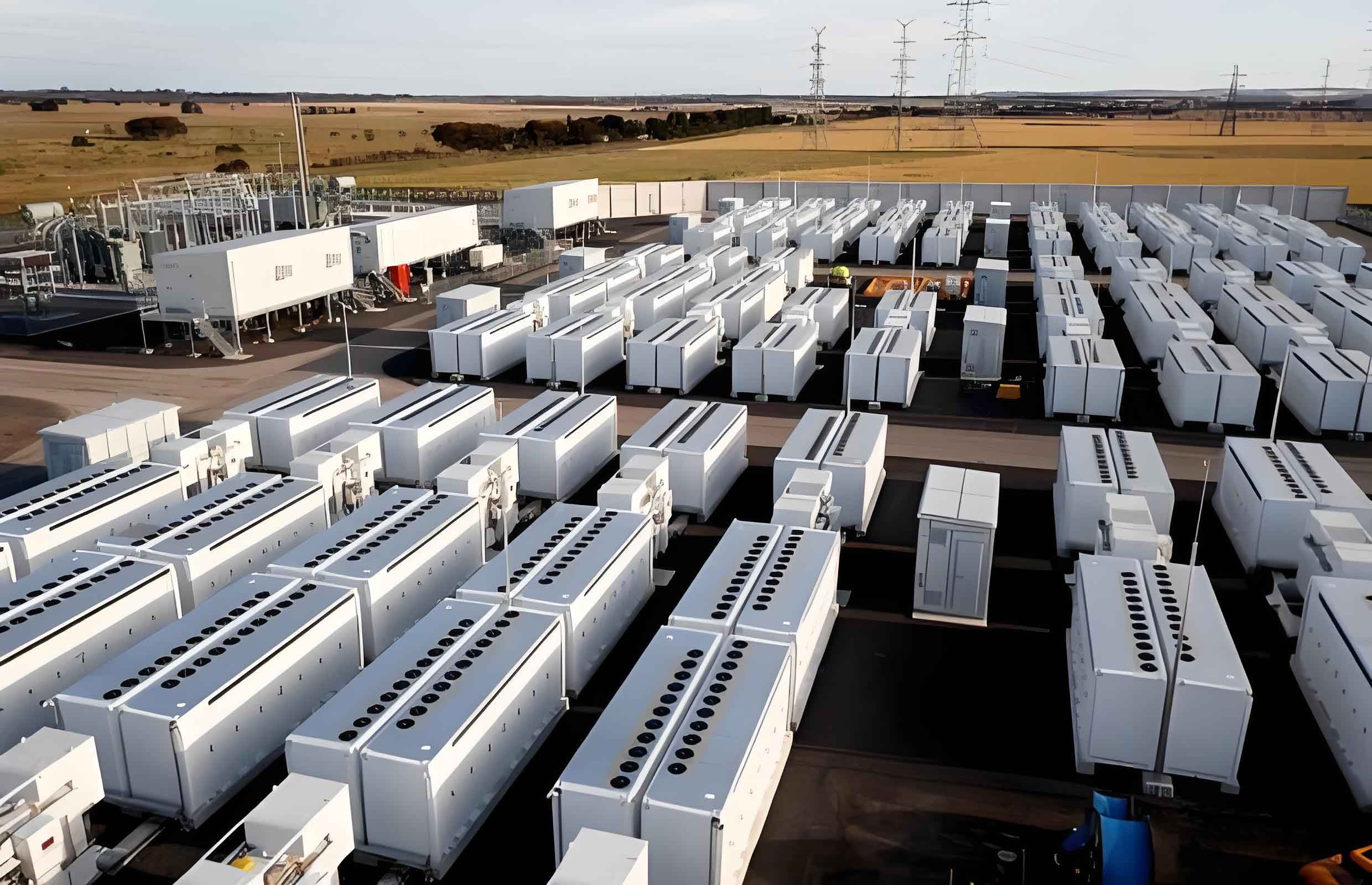
In the context of the global pursuit of carbon neutrality and peak carbon emissions, the integration of renewable energy into power grids has become a critical strategy for achieving a low-carbon energy transition. Energy storage systems, especially electrochemical energy storage, play an indispensable role in smoothing renewable energy fluctuations, providing fast response to load changes, and enhancing grid resilience. Among various storage technologies, lithium-ion batteries have gained widespread adoption due to their high energy density, high output power, long cycle life, and relatively low self-discharge rate. However, the thermal management of large-scale battery systems remains a significant technical challenge, particularly for containerized energy storage battery units where batteries are densely packed and generate substantial heat during operation. High operating temperatures can lead to accelerated capacity degradation, reduced lifespan, and severe safety risks such as thermal runaway. Therefore, designing a well-functioning thermal management system is essential to ensure the reliable, safe, and efficient operation of the entire energy storage battery plant.
In this paper, I present a comprehensive study on the design and optimization of a thermal management system for a large containerized energy storage battery system with a rated capacity of 1540 kWh. The work involves both one-dimensional system-level simulation and three-dimensional computational fluid dynamics (CFD) analysis. First, I establish a thermal model for lithium-ion cells and validate it against experimental data. Next, I design an all-weather cooling heat pump system that operates in three distinct modes depending on ambient temperature. Then, I conduct three-dimensional simulations to examine the airflow distribution and temperature uniformity within the battery enclosure. Finally, I optimize the supply air angle and return air vent location using the TOPSIS evaluation method, leading to significant improvements in cooling performance and temperature uniformity.
1. Thermal Behavior of Lithium-Ion Batteries
1.1 Structure and Working Principle
Lithium-ion batteries used in energy storage systems typically consist of positive and negative electrodes, current collectors, an electrolyte, a separator, and a metallic casing. The positive electrode is commonly made from lithium metal oxides such as LiFePO₄, LiCoO₂, or LiMn₂O₄, while the negative electrode is usually graphitic carbon. During charge, lithium ions are extracted from the positive electrode and inserted into the negative electrode through the electrolyte; during discharge, the opposite process occurs. This intercalation/deintercalation process generates heat due to internal resistance, electrochemical reactions, polarization, and side reactions.
1.2 Heat Generation Mechanisms
The total heat generated in a lithium-ion cell can be expressed as the sum of four contributions: Joule heat, reaction heat, polarization heat, and side-reaction heat. The overall heat generation rate is often described by the Bernardi equation:
\[
\Phi = I \left( E_0 – E \right) – I T \frac{dE_0}{dT}
\]
where \(I\) is the current, \(E_0\) is the open-circuit voltage, \(E\) is the operating voltage, \(T\) is the cell temperature, and \(dE_0/dT\) represents the entropy coefficient. The first term represents heat produced by internal resistance and polarization, while the second term represents reversible entropy heat.
For detailed modeling, the heat generation rate of the battery core can be calculated using:
\[
\Phi = I^2 R_e + I T \frac{dE_0}{dT}
\]
where \(R_e\) is the equivalent internal resistance. The positive and negative tabs also contribute additional Joule heating due to contact resistance and ohmic losses.
1.3 Thermal Properties and Transport
Because a battery is composed of many layers of different materials, its thermal conductivity is anisotropic. The effective thermal conductivities along different axes can be obtained using the series and parallel resistance analogy. The equivalent density and specific heat capacity are calculated by volume averaging:
\[
\rho_{\text{batt}} = \frac{\sum_i \rho_i V_i}{\sum_i V_i}, \quad C_{p,\text{batt}} = \frac{\sum_i \rho_i C_{p,i} V_i}{\sum_i \rho_i V_i}
\]
For the battery considered in this study (a 46 Ah, 3.2 V LiFePO₄ cell), the relevant properties are summarized in the table below.
| Parameter | Value |
|---|---|
| Density (kg/m³) | 2136.8 |
| Specific heat capacity (J/(kg·K)) | 1051.8 |
| Thermal conductivity – x direction (W/(m·K)) | 36.67 |
| Thermal conductivity – y direction (W/(m·K)) | 0.66 |
| Rated capacity (Ah) | 46 |
| Rated voltage (V) | 3.2 |
| Internal resistance (mΩ) | ≤ 0.2 |
| Dimension (mm) | 240 × 173 × 53 |
1.4 Simulation and Validation of the Battery Thermal Model
Using the AMEsim environment, I developed a lumped-parameter thermal model for a single cell. The model includes air convection heat transfer from the cell surface and internal uniform heat generation. Boundary conditions are set with the ambient air temperature at 25 °C and 35 °C, respectively. Simulations are performed for discharge rates of 1C, 1.5C, and 2C. Figure 1 shows the temperature evolution with time for different discharge rates at an ambient temperature of 25 °C. As the discharge rate increases, the temperature rise becomes more pronounced due to the higher heat generation rate relative to heat dissipation.
To validate the model, I compared the simulated surface temperature of a single cell during a 1.5C discharge at an ambient temperature of 25 °C with the experimentally measured values reported in a previous study. The comparison is shown in Figure 2. The maximum deviation between the simulation and experimental data is about 1.12 °C, corresponding to a relative error of 3.8%. This good agreement confirms that the proposed battery thermal model is accurate and suitable for further system-level simulations.
| Discharge rate | Ambient temp (°C) | Final battery temp (°C) | Temperature rise (°C) |
|---|---|---|---|
| 1C | 25 | 31.2 | 6.2 |
| 1.5C | 25 | 33.1 | 8.1 |
| 2C | 25 | 34.9 | 9.9 |
| 1C | 35 | 38.1 | 3.1 |
| 1.5C | 35 | 41.9 | 6.9 |
| 2C | 35 | 45.2 | 10.2 |
2. Design of the All-Weather Thermal Management System
2.1 System Overview
The containerized energy storage battery system studied here comprises two battery compartments, each containing two clusters of battery racks, with three racks per cluster and eight battery packs on each rack, giving a total of 48 battery packs per compartment. The system is cooled by forced air. To provide cooling year-round, I designed a composite refrigeration system that combines a heat pump loop with a water–glycol solution loop. The water–glycol solution acts as a secondary coolant in summer and as the direct refrigerant in winter, resolving the problem that conventional air conditioning systems cannot operate effectively at low ambient temperatures.
2.2 Operating Strategies
The thermal management system is configured for three distinct modes based on the outdoor temperature \(T_a\):
Mode 1 (Summer, \(T_a \ge 15\,^\circ\text{C}\)): The heat pump operates in a standard refrigeration cycle. The water–glycol solution circulates through the indoor heat exchanger (plate heat exchanger) to absorb heat from the battery compartment and reject it via the outdoor heat exchanger. This mode provides effective cooling during hot periods.
Mode 2 (Transition season, \(0\,^\circ\text{C} < T_a < 15\,^\circ\text{C}\)): A second outdoor heat exchanger is activated in the water–glycol loop to act as an auxiliary cooling device. The solution first rejects part of its heat to the ambient air in this heat exchanger, thereby reducing the load on the heat pump compressor. This improves system efficiency and compensates for the reduced performance of the heat pump at lower temperatures.
Mode 3 (Winter, \(T_a \le 0\,^\circ\text{C}\)): The system first operates in a preheating mode for 6000 seconds to bring the battery temperature above the minimum recommended level (10 °C). The four-way valve is switched so that the heat pump delivers hot refrigerant to the indoor heat exchanger, warming the water–glycol solution, which then heats the air in the battery compartment. After preheating, the heat pump compressor is switched off, and the water–glycol solution is circulated through the second outdoor heat exchanger to dissipate the battery heat directly to the cold ambient air. This “free cooling” method eliminates the need for compressor operation and provides an efficient solution for winter cooling.
2.3 Component Models
Key components of the thermal management system include the compressor, expansion valve, heat exchangers, water pump, and battery pack. In AMEsim, each component is represented by a lumped-parameter model that captures the essential thermodynamic behavior.
Compressor: The compressor model determines the mass flow rate and power consumption based on the displacement, rotational speed, and volumetric efficiency \(\eta_v\):
\[
\dot{m}_c = \eta_v \rho_{suc} N V_d
\]
where \(N\) is the rotational speed and \(V_d\) is the displacement volume. The isentropic efficiency \(\eta_s\) is used to calculate the enthalpy rise across the compressor.
Expansion valve: The expansion valve is modeled as an orifice with a variable opening. The refrigerant flow is expressed as:
\[
\dot{m}_v = k A \sqrt{2 \rho_{in} (p_{in} – p_{out})}
\]
where \(k\) is the flow coefficient, \(A\) is the effective area, and \(p_{in}\), \(p_{out}\) are the inlet and outlet pressures.
Heat exchangers: The outdoor heat exchangers (condenser in summer, evaporator in winter) and the indoor heat exchanger are modeled with effectiveness-NTU relations. For the plate heat exchanger used between the refrigerant and water–glycol solution, the heat transfer rates on both sides are calculated using appropriate correlations for single-phase and two-phase flows. The wall temperature is a state variable determined from the energy balance:
\[
\frac{dT_{wall}}{dt} = \frac{\Phi_i – \Phi_e}{m_{wall} C_{p,wall}}
\]
where \(\Phi_i\) and \(\Phi_e\) are the internal and external heat fluxes.
Water pump: The pump circulates the water–glycol solution. Its flow rate is determined by the pump characteristic curve and system resistance. The required cooling fluid flow rate is calculated from the maximum heat load:
\[
V_c = \frac{Q_{max}}{\rho_c C_{p,c} \Delta T_c}
\]
where \(\Delta T_c\) is the allowable temperature rise of the coolant.
3. One-Dimensional Simulation Results and Strategy Assessment
I performed one-dimensional simulations of the entire thermal management system under various ambient temperatures and discharge rates using AMEsim. The battery pack is modeled as a lumped thermal mass with heat generation calculated from the validated cell model. The control strategy uses the temperature of the battery pack closest to the return air vent (pack number 6 in my notation) as the feedback signal. The compressor speed, pump speed, and fan speed are adjusted to maintain the battery temperature below 35 °C.
3.1 Summer Operation
Figures 3 and 4 show the required airflow rate and the temperature response of battery pack 6 for different discharge rates at ambient temperatures of 35 °C and 25 °C, respectively. At \(T_a = 35\,^\circ\text{C}\), the initial cabin temperature is already above the set point, so the system immediately provides a high airflow rate. At 2.5C discharge, the required airflow reaches 7.06 kg/s, while at 1.0C it is about 0.78 kg/s. At \(T_a = 25\,^\circ\text{C}\), the system initially operates at minimal airflow until the battery temperature reaches 35 °C, after which the airflow increases proportionally. The time to reach the set point depends strongly on the discharge rate: at 1.0C it takes about 34.2 × 10³ s, whereas at 2.5C it is only 3.8 × 10³ s.
| Discharge rate | Time to reach 35 °C (s) at \(T_a=25\,^\circ\text{C}\) | Time to steady state (s) at \(T_a=35\,^\circ\text{C}\) |
|---|---|---|
| 1.0C | 34.2 × 10³ | 5.6 × 10³ |
| 1.5C | 13.5 × 10³ | 4.2 × 10³ |
| 2.0C | 6.8 × 10³ | 3.7 × 10³ |
| 2.5C | 3.8 × 10³ | 3.4 × 10³ |
From the temperature curves of the individual battery packs, the temperature decreases from pack 6 (near the return air vent) to pack 1 (near the supply air inlet). This is expected because the air temperature increases as it passes over the battery packs. The maximum temperature difference among the packs is about 3.66 °C at 1.0C discharge, which is within the recommended limit of 5 °C.
3.2 Transition Season Operation
In the transition season, the ambient temperature is lower, so the initial battery temperature is below the set point. The system runs at minimum airflow until the battery pack reaches 35 °C. With the auxiliary outdoor heat exchanger operating, the compressor load is reduced. At \(T_a=15\,^\circ\text{C}\), the time for the battery to reach 35 °C ranges from 12.8 × 10³ s at 1.0C to 3.3 × 10³ s at 2.5C. At \(T_a=5\,^\circ\text{C}\), the corresponding times increase to 71.4 × 10³ s and 6.5 × 10³ s respectively, due to the lower initial temperature and slower heating rate.
The data in Table 3 summarize the key performance metrics for different ambient temperatures at a discharge rate of 2.0C.
| Ambient temperature (°C) | Cooling capacity (kW) | Heating capacity (kW) | Power consumption (kW) | Time to steady state (s) |
|---|---|---|---|---|
| 35 | 33.76 | — | 10.64 | 3.7 × 10³ |
| 25 | 25.32 | — | 8.14 | 9.8 × 10³ |
| 15 | 15.32 | — | 4.95 | 14.5 × 10³ |
| 5 | 8.32 | — | 3.23 | 20.1 × 10³ |
| -5 | — | 8.92 | 3.96 | 19.8 × 10³ |
| -15 | — | 12.65 | 5.87 | 21.3 × 10³ |
3.3 Winter Operation
In winter, the battery pack is preheated to at least 10 °C before operation. The preheating phase lasts 6000 seconds, during which the heat pump operates in a heating mode. After preheating, the system switches to free cooling mode, using the second outdoor heat exchanger to reject heat to the ambient air. At \(T_a=-5\,^\circ\text{C}\), the battery temperature reaches the set point (35 °C) after about 13.4 × 10³ s for a 1.0C discharge and 3.8 × 10³ s for a 2.5C discharge. At \(T_a=-15\,^\circ\text{C}\), these times increase slightly to 14.7 × 10³ s and 4.2 × 10³ s, respectively. The maximum temperature difference among the battery packs remains below 5 °C under all conditions, satisfying the design target.
3.4 Strategy Adaptability
The simulation results demonstrate that the proposed thermal management system is capable of maintaining the maximum battery temperature below 35 °C and the temperature difference among packs below 5 °C for all operating scenarios considered. The use of the auxiliary outdoor heat exchanger in the transition season significantly reduces compressor power consumption, and the free-cooling mode in winter eliminates compressor usage entirely, greatly enhancing the overall system efficiency.
4. Three-Dimensional CFD Modeling and Optimization
4.1 Physical Model and Simplification
To further improve the cooling effectiveness of the thermal management system, I performed a three-dimensional CFD analysis of the battery compartment. The computational domain includes one of the two identical compartments, measuring 4760 mm × 1000 mm × 2700 mm. It contains two battery clusters, each composed of three racks with eight battery packs per rack. The battery packs are 570 mm × 570 mm × 230 mm. The supply air duct is located above the battery racks, with six rectangular outlets (340 mm × 140 mm) on the side wall of the duct. The return air vent is originally located on the right-side wall with dimensions 180 mm × 1000 mm. The geometry is shown schematically in Figure 5.
For the CFD simulation, I made the following assumptions:
- The battery materials are homogeneous and isotropic, with constant thermal properties.
- The heat generation rate is uniform within each battery pack.
- The container walls are adiabatic with no-slip condition.
- The airflow is steady, incompressible, and turbulent.
4.2 Governing Equations
The airflow and heat transfer are governed by the continuity, momentum, and energy equations. For turbulent flow, the standard k-ε model was adopted. The Reynolds number based on the supply air velocity (3.89 m/s) and the characteristic length is approximately 48,323, confirming turbulent flow. The governing equations are:
Continuity:
\[
\frac{\partial u_i}{\partial x_i} = 0
\]
Momentum:
\[
\frac{\partial}{\partial x_j} \left( \rho u_i u_j \right) = -\frac{\partial p}{\partial x_i} + \frac{\partial}{\partial x_j} \left[ \left( \mu + \mu_t \right) \frac{\partial u_i}{\partial x_j} \right]
\]
Air energy equation:
\[
\rho_a C_a \left( u \frac{\partial T}{\partial x} + v \frac{\partial T}{\partial y} + w \frac{\partial T}{\partial z} \right) = \nabla \cdot \left( k_{eff} \nabla T \right)
\]
Battery energy equation:
\[
\nabla \cdot \left( k_b \nabla T_b \right) + q_b = 0
\]
where \(q_b\) is the volumetric heat generation rate within the battery pack.
4.3 Boundary Conditions and Numerical Setup
The initial and boundary conditions are set as follows: the ambient temperature is 25 °C; the supply air temperature is 18 °C; the supply air velocity is 3.89 m/s; the return vents are treated as free outflow boundaries; the battery heat generation is 2408.76 W/m³; and the external walls are adiabatic. The convective heat transfer coefficient at the battery surfaces is set to 5 W/(m²·K). The SIMPLE algorithm is used for pressure-velocity coupling, with second-order upwind spatial discretization.
4.4 Mesh Independence Study
A structured hexahedral mesh was generated with local refinement near the battery surfaces and vent openings. Six mesh sizes were tested: 608,000; 1,023,000; 1,492,000; 1,932,000; 2,425,000; and 3,019,000 cells. The resulting average battery surface temperature and the average return air velocity were monitored. When the mesh exceeded 1.93 million cells, the change in both quantities was less than 2%, indicating mesh independence. Therefore, a mesh of about 1.93 million cells was used for the final simulations.
4.5 Model Validation
To validate the CFD model, I compared the predicted temperatures with the experimental data from a previous study on a forced-air-cooled lithium-ion battery module. In that experiment, a battery module containing ten prismatic cells was cooled by air at 3 m/s and an ambient temperature of 25 °C. The temperature at several monitoring points was measured. My simulation results were within 4.4% of the experimental values at all monitoring points, confirming the reliability of the present numerical model for predicting battery cooling performance.
5. Optimization of Supply Air Angle and Return Air Vent Location
5.1 Evaluation Metrics
To evaluate the airflow organization and thermal performance, I defined four dimensionless metrics:
1. Heat removal efficiency:
\[
\eta_t = \frac{T_e – T_s}{T_a – T_s}
\]
where \(T_e\) is the average exhaust air temperature, \(T_s\) is the supply air temperature, and \(T_a\) is the average air temperature in the compartment.
2. Temperature uniformity coefficient:
\[
\sigma_t = 1 – \frac{1}{2} \sqrt{\frac{\sum_{i=1}^n (T_i – \bar{T})^2}{n \cdot \bar{T}^2}}
\]
3. Velocity uniformity coefficient:
\[
\sigma_v = 1 – \frac{1}{2} \sqrt{\frac{\sum_{i=1}^n (v_i – \bar{v})^2}{n \cdot \bar{v}^2}}
\]
4. Air change efficiency:
\[
\eta_\alpha = \frac{\tau_n}{\tau_y} = \frac{V/G}{2\bar{\tau}}
\]
where \(V\) is the room volume, \(G\) is the supply air volume flow rate, and \(\bar{\tau}\) is the mean age of air.
5.2 TOPSIS Evaluation Method
TOPSIS (Technique for Order Preference by Similarity to an Ideal Solution) is a multi-criteria decision-making method. It ranks alternatives based on their geometric distance from the positive ideal solution (best possible performance) and the negative ideal solution (worst possible performance). The steps are:
- Construct the normalized decision matrix \(A = [a_{ij}]\), where \(a_{ij} = x_{ij} / \sqrt{\sum_{i=1}^m x_{ij}^2}\).
- Determine the positive ideal solution \(A^+\) and negative ideal solution \(A^-\).
- Calculate the distances \(D_i^+\) and \(D_i^-\) for each alternative.
- Compute the relative closeness \(S_i = D_i^- / (D_i^+ + D_i^-)\).
- Rank the alternatives according to \(S_i\), with the highest value being the best.
5.3 Effect of Supply Air Angle
Starting with a base case of 45°, I simulated supply air angles of 30°, 60°, 75°, and 90° (measured from the vertical). The original return air vent was located on the right-side wall at Z = 0.80 m. The velocity and temperature fields were examined at the vertical plane Y = 3.56 m.
As the supply air angle increases from 30° to 90°, the airflow pattern changes significantly. At smaller angles, the air has a larger vertical velocity component, causing it to descend rapidly along the divider wall and reducing the amount of air that penetrates the battery racks. At larger angles, the horizontal momentum is higher, and the air impinges on the divider wall, creating a high-pressure zone in the upper region. This promotes better diffusion of the air across the entire battery cluster, leading to more uniform flow and enhanced heat transfer.
Figure 6 shows the temperature distribution on the battery pack surfaces for different supply air angles. The hottest packs are consistently located near the lower-left side (D-7 pack) due to the lower static pressure in that region. At 30°, the maximum temperature reaches 41.59 °C; at 90°, it drops to 33.58 °C, a reduction of 19.5%. The average temperature difference among all packs decreases from 4.12 °C to 3.46 °C, showing improved temperature uniformity.
| Supply air angle | \(\sigma_t\) | \(\sigma_v\) | \(\eta_t\) | \(\eta_\alpha\) |
|---|---|---|---|---|
| 30° | 0.944 | 0.890 | 1.088 | 0.441 |
| 45° | 0.946 | 0.856 | 1.052 | 0.578 |
| 60° | 0.951 | 0.806 | 1.078 | 0.755 |
| 75° | 0.953 | 0.784 | 1.083 | 0.843 |
| 90° | 0.954 | 0.773 | 1.091 | 0.875 |
Applying TOPSIS to these metrics, I found that the 90° angle provides the best overall performance, with a relative closeness value of 0.30, followed by 75° (0.29), 60° (0.22), 45° (0.08), and 30° (0.11). Therefore, a supply angle of 90° was selected as the optimal configuration for the subsequent return air vent optimization.
5.4 Effect of Return Air Vent Location
With the supply air angle fixed at 90°, I evaluated five different return air vent configurations, as summarized in the table below. The original configuration (Case 1) has a single large return on the right wall at Z = 0.80 m. Case 2 places the same vent lower at Z = 0.25 m. Cases 3–5 replace the single vent with six smaller vents (340 mm × 140 mm) distributed along the fire-door side wall at different heights: Z = 0.25 m, 0.85 m, and 1.35 m.
| Case | Return vent size | Location |
|---|---|---|
| Case 1 | 0.28 m × 1.00 m (single) | Right side wall, Z=0.80 m |
| Case 2 | 0.28 m × 1.00 m (single) | Right side wall, Z=0.25 m |
| Case 3 | 0.34 m × 0.14 m (six) | Fire-door side, Z=0.25 m |
| Case 4 | 0.34 m × 0.14 m (six) | Fire-door side, Z=0.85 m |
| Case 5 | 0.34 m × 0.14 m (six) | Fire-door side, Z=1.35 m |
The velocity vector fields at Y = 3.56 m clearly show that the original right-wall return creates a strong flow toward the right side, leaving the left cluster relatively stagnant. By contrast, when the return vents are placed on the fire-door side, the low-pressure zone is distributed more uniformly across the racks, promoting a more even airflow through the battery packs. Lowering the return vents (Case 3) causes air to short-circuit through the lower part of the racks, while raising them too high (Case 5) starves the lower packs.
The temperature distribution on the battery surfaces for all cases is shown in Figure 7. Case 4, with the return vents evenly spaced at Z = 0.85 m on the fire-door side, yields the most uniform temperature distribution. The max surface temperature drops from 33.75 °C (Case 1) to 30.02 °C, and the overall temperature uniformity improves significantly. The average temperature difference among all measured points in Case 4 is 3.01 °C, a 21.4% reduction compared to Case 1. The system resistance also decreases from 26.83 Pa to 21.82 Pa, indicating a lower fan power requirement.
| Case | \(\sigma_t\) | \(\sigma_v\) | \(\eta_t\) | \(\eta_\alpha\) |
|---|---|---|---|---|
| Case 1 | 0.954 | 0.773 | 1.091 | 0.875 |
| Case 2 | 0.955 | 0.781 | 1.111 | 0.896 |
| Case 3 | 0.966 | 0.818 | 1.635 | 0.960 |
| Case 4 | 0.968 | 0.803 | 1.763 | 0.978 |
| Case 5 | 0.965 | 0.839 | 1.656 | 0.957 |
The TOPSIS evaluation results are listed below. Case 4 obtains the highest relative closeness (0.35), outperforming the other configurations. Thus, the optimal return air vent arrangement is six evenly distributed vents on the fire-door side at Z = 0.85 m, combined with a supply air angle of 90°.
| Case | \(D_i^+\) | \(D_i^-\) | \(S_i\) | Rank |
|---|---|---|---|---|
| Case 1 | 0.212 | 0.001 | 0.01 | 5 |
| Case 2 | 0.203 | 0.013 | 0.02 | 4 |
| Case 3 | 0.041 | 0.171 | 0.30 | 3 |
| Case 4 | 0.019 | 0.210 | 0.35 | 1 |
| Case 5 | 0.034 | 0.179 | 0.32 | 2 |
Compared with the original design (Case 1 with 45° angle), the optimized system (Case 4 with 90° angle) reduces the maximum battery surface temperature from 36.67 °C to 30.63 °C, a decrease of 16.47%. The average temperature difference among the battery surfaces is reduced by 21.4%, from 3.83 °C to 3.01 °C. This substantial improvement is mainly attributed to the better airflow distribution achieved by the louvered supply vents and the uniformly positioned return vents, which eliminate the stagnant zones in the lower left region of the battery compartment.
6. Conclusions
In this paper, I have presented a comprehensive design and optimization study for a thermal management system of a 1540 kWh containerized energy storage battery. The key findings are summarized as follows:
- A validated lithium-ion battery thermal model was developed, which accurately predicts cell temperature evolution under various discharge rates and ambient temperatures.
- An all-weather thermal management system incorporating a heat pump and a water–glycol secondary loop was designed. The system operates in three modes and successfully maintains the maximum battery temperature below 35 °C and the temperature difference among battery packs below 5 °C across all simulated ambient conditions.
- Three-dimensional CFD simulations were used to analyze the airflow and temperature fields inside the battery compartment. The model was validated against experimental data from the literature.
- Increasing the supply air angle from 30° to 90° improved airflow distribution and reduced the maximum battery pack temperature from 41.59 °C to 33.58 °C. The TOPSIS evaluation confirmed 90° as the optimal angle.
- Relocating the return air vents from the right wall to the fire-door side at an intermediate height (Z = 0.85 m) significantly improved temperature uniformity. The optimal configuration (Case 4) reduced the maximum battery surface temperature by 16.47% and the average temperature difference by 21.4% compared to the original design.
The findings of this study provide valuable insights into the design and optimization of thermal management systems for large-scale containerized energy storage battery installations. The combination of louvered supply vents and uniformly distributed return vents proves to be an effective strategy for enhancing cooling performance and temperature uniformity, thereby contributing to the reliability and safety of energy storage battery systems.