
I have dedicated this thesis to exploring how battery energy storage can effectively assist thermal power units in secondary frequency regulation of modern power systems. With the rapid integration of renewable energy sources, the frequency stability of the power grid faces unprecedented challenges. Traditional thermal power units, with their relatively slow response speed and limited regulation flexibility, are no longer sufficient to guarantee grid frequency quality. Battery energy storage systems, characterized by millisecond response time and high regulation accuracy, have become a promising complementary resource. The objective of my research is to develop a comprehensive control strategy that allocates frequency regulation commands between the thermal plant and the battery energy storage system in an optimal manner, ensuring both technical performance and economic feasibility.
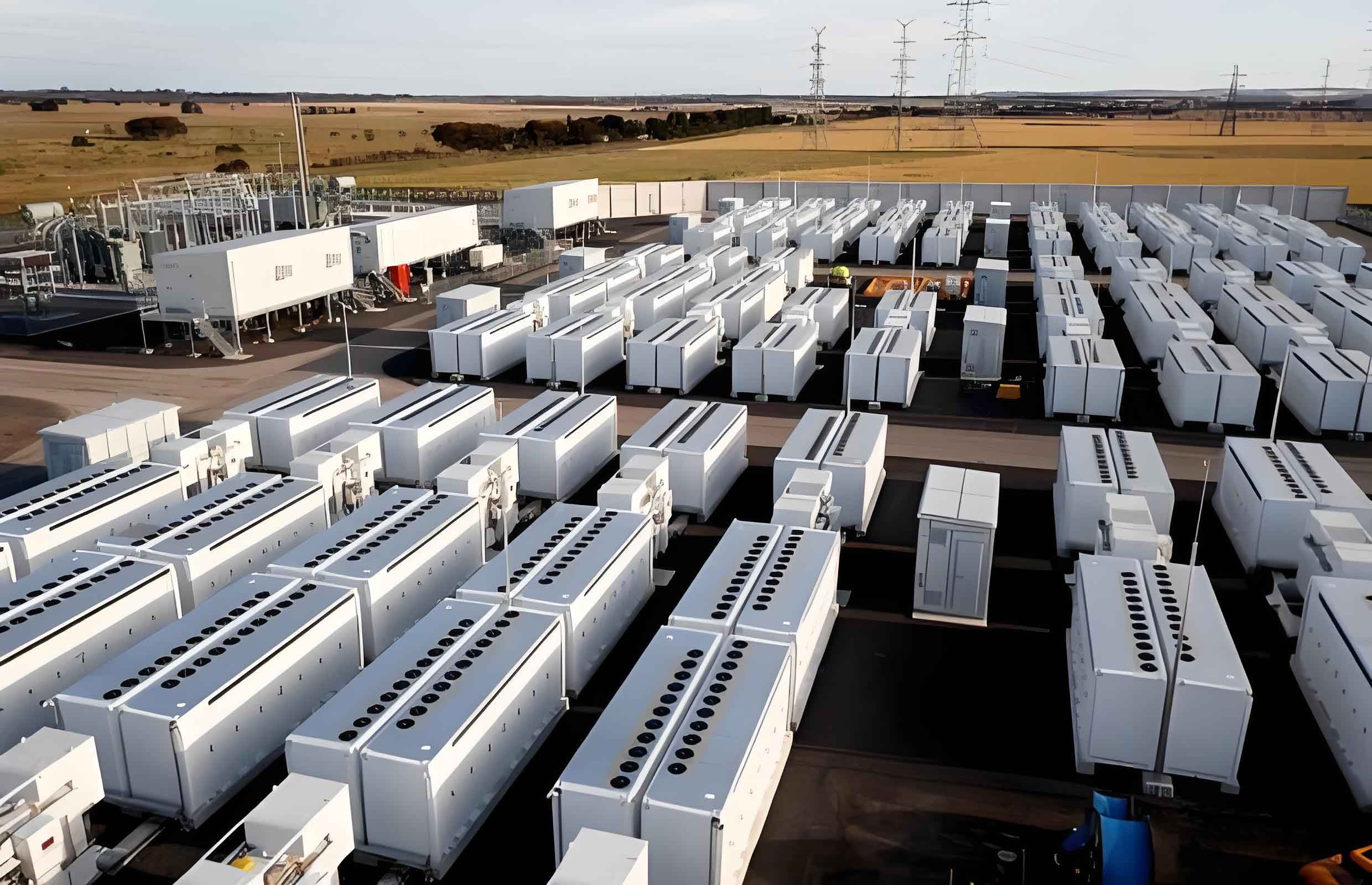
I first analyze the development status of battery energy storage. In recent years, many demonstration projects across the globe have deployed battery energy storage for grid frequency regulation. Some representative projects are summarized in the following table.
| Country | Project | Storage capacity | Type | Operation date |
|---|---|---|---|---|
| USA | Moss Landing BESS | 300MW/1200MWh | Lithium-ion | Dec. 2020 |
| China | Wuhai Thermal Power Plant BESS | 6MW/3MWh | Lithium-ion | Sep. 2020 |
| UK | Mendi Power Storage | 44.9MW/99.8MWh | Lithium-ion | Dec. 2021 |
| China | Yueqing Power Plant | 20MW/20MWh | LFP | Sep. 2022 |
| China | Huaneng Yuhuan | 30MW/30MWh | LFP | Sep. 2022 |
| China | Yangxi Power Plant | 52.5MW/55.9MWh | LFP | Dec. 2024 |
From the existing literature, I have identified three key research directions: (1) the optimal allocation of frequency regulation commands between thermal units and battery energy storage; (2) the state of charge (SOC) equalization and sustainable operation of the battery storage; and (3) the economic evaluation of the storage-assisted frequency regulation service. My work addresses all three aspects by proposing an improved variational mode decomposition (VMD) method, a double-layer fuzzy control architecture, and a comprehensive cost-benefit analysis model.
Fundamental Principles of Power System Frequency Regulation
Power system frequency regulation is essential for maintaining the balance between generation and load. When the load changes, the system frequency deviates from its nominal value. The relationship between the load change and the frequency deviation can be expressed by the frequency characteristic of the load. For a typical load, the active power consumption is a function of the system frequency:
$$P_{L}=P_{LN}\left(\alpha_0+\alpha_1 \frac{f}{f_N}+\alpha_2 \left(\frac{f}{f_N}\right)^2+\cdots\right) \tag{1}$$
where \(P_L\) and \(P_{LN}\) are the load active power at frequency \(f\) and at rated frequency \(f_N\), respectively, and \(\alpha_i\) are the proportional coefficients. The load-frequency coefficient is defined as:
$$K_D=\frac{\Delta P_L}{\Delta f} \tag{2}$$
For a generating unit, its frequency regulation characteristic is described by:
$$\Delta P_G=-\frac{1}{\sigma}\frac{\Delta f}{f_N}=-\left|K_G\right|\Delta f \tag{3}$$
where \(K_G\) is the unit regulation power and \(\sigma\) is the per-unit speed droop.
Primary frequency control is a local automatic control that responds to frequency deviations through governor action. It is a static regulation method and inevitably leaves a steady-state frequency error. Secondary frequency control, also called automatic generation control (AGC), adjusts the active power setpoints of the participating generators to restore both the frequency and the inter-area power exchange to their scheduled values. In an interconnected area control system, the area control error (ACE) is used as the control input. When the tie-line bias control (TBC) mode is adopted, the ACE is defined as:
$$\text{ACE}=B\Delta f+\Delta P_{\text{tie}} \tag{4}$$
where \(B\) is the frequency bias coefficient and \(\Delta P_{\text{tie}}\) is the deviation of the tie-line power exchange.
To simulate the dynamic response of the thermal power plant, I have constructed a model for each component. The governor is represented by a first-order inertia as:
$$G_{\text{gov}}(s)=\frac{1}{1+sT_{\text{G}}} \tag{5}$$
For the non-reheat steam turbine, the transfer function is:
$$G_{\text{T}}(s)=\frac{1}{1+sT_{\text{CH}}} \tag{6}$$
The generator-load dynamic characteristic is described by:
$$G_{\text{gen-load}}(s)=\frac{1}{2Hs+D} \tag{7}$$
where \(H\) is the inertia constant and \(D\) is the load damping coefficient. The tie-line model between two areas is:
$$\Delta P_{\text{tie},i}(s)=\frac{T_{12}}{s}\left(\Delta \omega_i(s)-\Delta \omega_j(s)\right) \tag{8}$$
where \(T_{12}\) is the synchronizing torque coefficient of the tie-line.
For the battery energy storage system (BESS), I adopt an equivalent first-order lag model to capture its fast response characteristics:
$$G_{\text{BESS}}(s)=\frac{1}{1+sT_{\text{b}}} \tag{9}$$
where \(T_{\text{b}}\) is the response time constant of the BESS. The state of charge (SOC) of the battery is governed by:
$$\text{SOC}(t)=\text{SOC}(t_0)-\frac{\int_{t_0}^{t} P_{\text{BESS}}(\tau)\,d\tau}{E_{\text{rated}}} \tag{10}$$
where \(E_{\text{rated}}\) is the rated energy capacity of the battery. By incorporating the BESS model into the two-area interconnected power system, I have established the complete frequency regulation model with the battery storage as an auxiliary control unit.
Improved VMD for Frequency Regulation Command Decomposition
Variational mode decomposition (VMD) is a powerful signal processing technique that decomposes a non-stationary signal into a set of band-limited intrinsic mode functions. I have used VMD to separate the ACE signal into high-frequency and low-frequency components, so that the high-frequency part can be assigned to the battery energy storage and the low-frequency part to the thermal units.
VMD solves a constrained variational problem to obtain the mode functions \(u_k(t)\) and their corresponding center frequencies \(\omega_k\). The constrained optimization problem is:
$$\min_{\{u_k\},\{\omega_k\}}\left\{\sum_k \left\| \partial_t \left[ \left(\delta(t)+\frac{j}{\pi t}\right) * u_k(t)\right] e^{-j\omega_k t}\right\|_2^2\right\} \quad \text{s.t.} \quad \sum_k u_k(t)=f(t) \tag{11}$$
where \(f(t)\) is the input signal and the star denotes convolution. By introducing the quadratic penalty factor \(\alpha\) and the Lagrangian multiplier \(\lambda\), the augmented Lagrangian is:
$$\mathcal{L}(\{u_k\},\{\omega_k\},\lambda)=\alpha \sum_k \left\| \partial_t \left[ \left(\delta(t)+\frac{j}{\pi t}\right) * u_k(t)\right] e^{-j\omega_k t}\right\|_2^2 + \left\| f(t)-\sum_k u_k(t)\right\|_2^2 + \left\langle \lambda(t), f(t)-\sum_k u_k(t)\right\rangle \tag{12}$$
The alternating direction method of multipliers (ADMM) is used to update \(u_k\) and \(\omega_k\) iteratively. The updating formulas are:
$$\hat{u}_k^{n+1}(\omega)=\frac{\hat{f}(\omega)-\sum_{i\neq k}\hat{u}_i(\omega)+\hat{\lambda}(\omega)/2}{1+2\alpha(\omega-\omega_k)^2} \tag{13}$$
$$\omega_k^{n+1}=\frac{\int_0^\infty \omega \left|\hat{u}_k(\omega)\right|^2 d\omega}{\int_0^\infty \left|\hat{u}_k(\omega)\right|^2 d\omega} \tag{14}$$
However, the performance of VMD heavily depends on two parameters: the decomposition mode number \(K\) and the penalty factor \(\alpha\). Conventionally these parameters are set empirically, which may lead to mode mixing or information loss. To overcome this limitation, I have developed a parameter optimization scheme.
First, I optimize the mode number \(K\) by using the Schmidt orthogonalization and residual minimization. After an initial decomposition with a candidate \(K\), the obtained modes are orthogonalized using the Schmidt orthogonalization process. The residual between the original signal and the sum of the orthogonalized modes is computed as:
$$r(t)=f(t)-\sum_{k=1}^{K} u_k^{\text{orth}}(t) \tag{15}$$
I select the value of \(K\) that yields the smallest residual energy. This ensures that the decomposed modes preserve the original signal information with minimal loss and that the modes have good orthogonality.
Second, I optimize the penalty factor \(\alpha\) using the sparrow search algorithm (SSA). The objective function is the orthogonality index (IO) of the decomposed modes, defined as:
$$IO=\frac{1}{2}\sum_{t=0}^{T}\sum_{h=1}^{n}\sum_{\substack{k=1 \\ k\neq h}}^{n}\frac{c_h(t)c_k(t)}{X^2(t)} \tag{16}$$
where \(X(t)\) is the original signal, \(c_k(t)\) are the IMFs, \(T\) is the signal duration, and \(n\) is the number of modes. A smaller IO indicates better orthogonality among the IMFs. Sparrow search algorithm is a swarm intelligence optimization method known for its strong global search capability and fast convergence. In my implementation, the population size is set to 60 and the maximum iteration number is 100. I compare SSA with particle swarm optimization (PSO) and whale optimization algorithm (WOA). The convergence curves show that SSA achieves a much lower fitness value and converges faster than the other two algorithms.
| IMF | Kurtosis with empirical parameters | Kurtosis with optimized parameters | Skewness with empirical parameters | Skewness with optimized parameters |
|---|---|---|---|---|
| IMF1 | 30.653 | 34.577 | 5.094 | 4.788 |
| IMF2 | 38.204 | 41.437 | 5.511 | 5.300 |
| IMF3 | 35.344 | 37.739 | 5.540 | 5.360 |
| IMF4 | 40.835 | 43.304 | 5.810 | 5.650 |
| IMF5 | 28.784 | 29.138 | 4.952 | 4.908 |
| IMF6 | 31.359 | 34.050 | 5.292 | 5.067 |
| IMF7 | 35.964 | 43.147 | 5.852 | 5.367 |
| IMF8 | 24.326 | 31.506 | 4.926 | 4.382 |
| IMF9 | 22.689 | 24.608 | 4.356 | 4.180 |
| IMF10 | 17.082 | 19.193 | 3.878 | 3.575 |
The experimental results demonstrate that the optimized VMD significantly reduces the modal mixing phenomenon. The kurtosis of the optimized IMFs is substantially higher, indicating that each mode has a sharper and more concentrated frequency spectrum, while the skewness is closer to zero, meaning the spectra are more symmetric. Therefore, the optimized VMD provides a more accurate decomposition of the ACE signal.
Secondary Frequency Regulation Control Strategy with Battery Energy Storage
After obtaining the optimized VMD, I can decompose the ACE signal into several IMFs. The high-frequency and low-frequency components are separated by analyzing the energy entropy of the IMFs. The energy of each IMF is calculated as:
$$E_i=\sum_{t=1}^{N} |c_i(t)|^2 \tag{17}$$
where \(N\) is the number of sampling points. The normalized energy weight is:
$$\bar{E}_i=\frac{E_i}{\sum_{k=1}^{K} E_k} \tag{18}$$
The energy change between adjacent IMFs is defined as:
$$\Delta c(i)=|\bar{E}_{i+1}-\bar{E}_i| \tag{19}$$
I choose the index \(n\) that gives the maximum \(\Delta c(i)\) as the boundary between the high-frequency and low-frequency parts. The low-frequency component, composed of the first \(n-1\) IMFs, is assigned as the power command to the thermal power units:
$$P_{\text{L}}=\sum_{i=1}^{n-1} c_i(t) \tag{20}$$
and the high-frequency component from the remaining IMFs is assigned to the battery energy storage:
$$P_{\text{H}}=\sum_{i=n}^{K} c_i(t) \tag{21}$$
In my implementation, the maximum energy change occurred between IMF7 and IMF8, so the initial filter order is set to \(n=7\). This means that IMF1-7 form the low-frequency command for the thermal units, and IMF8-10 constitute the high-frequency command for the battery storage.
To further optimize the power sharing, I have designed a double-layer fuzzy control architecture. The first layer fuzzy controller regulates the output power of the battery storage based on the high-frequency command and the real-time SOC. The inputs are the standardized high-frequency power \(\bar{P}_{\text{H}}\) and the SOC. The output is the smoothed power correction \(P_{\text{ess}}\). The fuzzy rules are designed according to the following principles: when the SOC is low, the discharging power is reduced and charging is encouraged; when the SOC is high, discharging is prioritized and charging is limited; when the SOC is in the normal range, the battery can follow the power command more freely. The membership functions for the inputs and output are Gaussian functions. The output surface of the fuzzy controller shows a smooth nonlinear relationship between the inputs and the output, allowing the battery to adapt its charging/discharging behavior according to its state.
The second layer fuzzy controller adaptively updates the VMD filtering order \(n\) based on the ultra-short-term load forecast and the battery output power. The inputs are the forecast load change \(\Delta P_{\text{load}}\) and the battery output \(P_{\text{ess}}\). The output is the adjustment to the filter order. The control logic is as follows: if the forecast load is expected to increase, the system should reserve more capacity in the battery storage; hence the filter order is increased to make the storage undertake less high-frequency component and reduce its current output. Conversely, if the load is expected to decrease, the filter order is decreased so that the battery contributes more to frequency regulation at the present time. This predictive adjustment enhances the adaptability of the control strategy and avoids excessive battery power fluctuations.
The overall control structure of the battery energy storage participating in secondary frequency regulation is presented in the following block diagram (formulated through the model equations described earlier). The system includes the thermal governor, the turbine, the generator-load dynamics, the tie-line model, the BESS model, and the two-layer fuzzy controllers.
| Parameter | Value | Parameter | Value |
|---|---|---|---|
| \(M_1\) | 10 | \(K_2\) | 20 |
| \(D_1\) | 1 | \(T_{12}\) | 0.87 |
| \(K_{P1}\) | -0.822 | \(T_{\text{CH}}\) | 0.3 |
| \(K_{I1}\) | -0.16 | \(T_{\text{b}}\) | 0.01 |
| \(K_{P2}\) | -0.822 | \(B_1\) | 21 |
| \(K_{I2}\) | -0.16 | \(B_2\) | 21 |
| \(T_{\text{G1}}\) | 0.086 | \(M_2\) | 10 |
| \(T_{\text{G2}}\) | 0.06 | \(D_2\) | 1 |
I have carried out simulations in MATLAB/Simulink on a two-area interconnected power system model. The rated power of each area is 1000 MW, the ramping rate of the thermal unit is 30 MW/min, and the AGC reserve capacity is from \(-50\) MW to \(50\) MW. The battery storage is rated at 10 MW/10 MWh, with an initial SOC of 0.5. Three control strategies are compared: Strategy 1 (thermal unit only without battery storage), Strategy 2 (single-layer fuzzy control with a fixed VMD filter order), and Strategy 3 (the proposed double-layer fuzzy control with adaptive filtering order).
The simulation results are evaluated using the maximum frequency deviation \(\Delta f_{\max}\), the steady-state frequency deviation \(\Delta f_s\), the initial rate of frequency decline \(V_m\), the frequency recovery rate \(V_r\), and the root-mean-square error of SOC (RMSE-SOC). The results are summarized in the following table.
| Evaluation index | Strategy 1 | Strategy 2 | Strategy 3 |
|---|---|---|---|
| \(\Delta f_{\max}\) (Hz) | 0.011718 | 0.0082136 | 0.0072817 |
| \(\Delta f_s\) (Hz) | 0.00351 | 0.00312 | 0.00302 |
| \(V_m\) (Hz/min) | 0.00198 | 0.00154 | 0.00136 |
| \(V_r\) (Hz/min) | \(8.38\times10^{-6}\) | \(5.38\times10^{-5}\) | \(6.73\times10^{-5}\) |
| RMSE-SOC | — | 0.0897 | 0.0877 |
From the table, one can observe that Strategy 2 and Strategy 3 significantly outperform Strategy 1, confirming that the battery energy storage can effectively improve the frequency regulation performance. When comparing Strategy 3 with Strategy 2, the proposed double-layer fuzzy control achieves a smaller maximum frequency deviation, a faster frequency recovery rate, and a lower RMSE-SOC. This indicates that the adaptive filter order helps the battery maintain a more stable SOC, reducing the risk of overcharge or overdischarge. The battery output curve under Strategy 3 is also smoother, which reduces mechanical wear on the thermal unit and extends the lifespan of the battery energy storage. Moreover, the tie-line power exchange deviation is reduced, indicating a more balanced load sharing between the control areas.
Economic Analysis of Battery Energy Storage Participating in AGC Frequency Regulation
To evaluate the economic viability of the proposed control strategy, I have established a comprehensive life-cycle cost-benefit model for the battery energy storage system. First, I analyze the existing frequency regulation compensation standards. In many regions, the compensation for the combined thermal-storage frequency regulation is based on the comprehensive regulation performance index \(K_P\), which is the product of three sub-indices: regulation rate \(K_1\), regulation accuracy \(K_2\), and response time \(K_3\). The compensation payment is then calculated as:
$$B_{K_P}=M_{\text{AGC}}\sum_{d=1}^{N} K_P \beta_d D_d \tag{22}$$
where \(M_{\text{AGC}}\) is the compensation standard per unit of regulation, \(D_d\) is the regulation depth of the \(d\)-th action, and \(\beta_d\) is the reversal coefficient. However, this compensation mechanism does not reflect the environmental benefit of the battery storage. Therefore, I propose a more advanced model that includes environmental benefits and can calculate the independent contribution of the battery energy storage.
I first model the battery life decay. The number of cycle life \(N_C\) as a function of depth of discharge (\(DOD\)) can be fitted as:
$$N_C(D_i)=N_{\text{L}}\cdot \left(\frac{D_i}{D_{\text{N}}}\right)^{-1.69}\exp\left(0.19\frac{D_i}{D_{\text{N}}}\right) \tag{23}$$
where \(D_{\text{N}}\) is the rated discharge depth (typically 1), \(N_{\text{L}}\) is the maximum number of cycles at the rated depth (set to 8000), and \(D_i\) is the depth of the \(i\)-th discharge cycle. The equivalent cycling coefficient that converts a partial cycle to an equivalent full cycle is:
$$\delta(D_i)=\frac{N_C(1)}{N_C(D_i)} \tag{24}$$
The daily equivalent full cycles \(N_d\) are obtained by summing the equivalent cycles of all charge-discharge events in a day, typically counted by the rain-flow counting method. The battery lifetime in years is then:
$$T_{\text{life}}=\frac{N_C(1)}{365 N_d} \tag{25}$$
The life-cycle cost of the battery storage consists of four components: investment cost, operation and maintenance (O&M) cost, replacement cost, and disposal cost. The annualized investment cost is:
$$C_{\text{inv}}=(C_{\text{bat.p}}P_{\text{rated}}+C_{\text{bat.e}}E_{\text{rated}})\cdot \frac{i(1+i)^{T_m}}{(1+i)^{T_m}-1} \tag{26}$$
where \(C_{\text{bat.p}}\) and \(C_{\text{bat.e}}\) are the unit power cost and unit energy cost of the battery, respectively, \(i\) is the discount rate (8%), and \(T_m\) is the project lifetime (20 years). The annual O&M cost is:
$$C_{\text{om}}=C_{\text{bat.pm}}P_{\text{rated}}+C_{\text{bat.em}}E_{\text{rated}} \tag{27}$$
where \(C_{\text{bat.pm}}\) and \(C_{\text{bat.em}}\) are the annual unit costs for power and capacity maintenance. The replacement cost accounts for future battery replacements, considering the annual decline in battery cost. The disposal cost includes the decommissioning and recycling expenses.
The total annualized life-cycle cost is computed as:
$$C_{\text{LCC}}=C_{\text{inv}}+C_{\text{om}}+C_{\text{rep}}+C_{\text{scr}} \tag{28}$$
On the benefit side, I consider three revenue streams: real-time electricity revenue, fuel-saving benefit, and environmental benefit. The real-time electricity revenue comes from the charging and discharging behavior of the battery during frequency regulation. The daily electricity revenue is computed as:
$$R_{\text{ele,d}}=\sum_{t=1}^{24}\sum_{n=1}^{60} R_{\text{ele},t} P_n \tag{29}$$
where \(R_{\text{ele},t}\) is the electricity price in hour \(t\), and \(P_n\) is the battery output power at minute \(n\) (positive when discharging, negative when charging). The annual electricity revenue is \(R_{\text{ele}}=300R_{\text{ele,d}}\), assuming 300 operating days per year.
The fuel-saving benefit arises from the fact that the battery shares the regulation burden, causing the thermal unit to reduce its output variation and thereby saving coal consumption. The annual fuel-saving benefit is:
$$R_{\text{fuel}}=\sum_{t=1}^{365} E_t C_{\text{fuel}} W_{\text{fuel}} \tag{30}$$
where \(E_t\) is the electrical energy discharged during frequency regulation on day \(t\), \(C_{\text{fuel}}\) is the coal price per unit, and \(W_{\text{fuel}}\) is the standard coal consumption per unit of electricity. The environmental benefit comes from the reduction of pollutant emissions, including nitrogen oxides (\(\mathrm{NO_x}\)), carbon dioxide (\(\mathrm{CO_2}\)), and sulfur dioxide (\(\mathrm{SO_2}\)):
$$R_{\text{eco}}=\sum_{t=1}^{365} E_t \left(C_{\mathrm{NO_x}}+C_{\mathrm{CO_2}}+C_{\mathrm{SO_2}}\right) \tag{31}$$
where \(C_{\mathrm{NO_x}}\), \(C_{\mathrm{CO_2}}\), and \(C_{\mathrm{SO_2}}\) are the environmental treatment costs per unit of emitted pollutants. The total annual benefit of the battery energy storage is:
$$R_{\text{total}}=R_{\text{ele}}+R_{\text{fuel}}+R_{\text{eco}} \tag{32}$$
I use the parameters listed in the following table to evaluate the economic performance of the proposed control strategy.
| Parameter | Value |
|---|---|
| \(C_{\text{bat.p}}\) (万元/MW) | 50 |
| \(C_{\text{bat.e}}\) (万元/MWh) | 120 |
| \(C_{\text{bat.pm}}\) (万元/MW) | 6 |
| \(C_{\text{bat.em}}\) (万元/MWh) | 0.1 |
| \(C_{\text{bat.ps}}\) (万元/MW) | 0.72 |
| \(C_{\text{bat.es}}\) (万元/MWh) | 0.72 |
| \(C_{\text{fuel}}\) (元/t) | 400 |
| \(W_{\text{fuel}}\) (g/MWh) | 350 |
| \(C_{\mathrm{NO_x}}\) (元/MWh) | 10.074 |
| \(C_{\mathrm{CO_2}}\) (元/MWh) | 18.669 |
| \(C_{\mathrm{SO_2}}\) (元/MWh) | 2.671 |
I compare the proposed double-layer fuzzy control strategy (Strategy 3) with the single-layer fuzzy control strategy (Strategy 2) in terms of economic indicators. The results are summarized below.
| Indicator | Strategy 2 | Strategy 3 |
|---|---|---|
| Annual average cost (万元) | 674.702 | 635.106 |
| Annual average profit (万元) | 96.804 | 116.163 |
| Battery replacement times over project duration | 9.644 | 9.187 |
| Battery operating life (years) | 1.8789 | 1.9631 |
The results show that the proposed double-layer fuzzy control strategy can reduce the annual cost, increase the annual profit, reduce the number of battery replacements, and extend the battery service life. This is because the adaptive filter order and the SOC-conscious power smoothing prevent the battery from experiencing excessive depth of discharge, thereby slowing down the ageing process. The economic benefits of the battery energy storage system are hence more attractive, which further justifies the integration of battery energy storage into secondary frequency regulation.
Conclusion
In this thesis, I have systematically studied the control strategy and economic performance of a battery energy storage system assisting thermal power units in secondary frequency regulation. I have drawn the following conclusions:
- The improved VMD method, with the mode number optimized by residual minimization and the penalty factor optimized by the sparrow search algorithm, can effectively reduce mode mixing and improve the decomposition accuracy of the ACE signal.
- The proposed double-layer fuzzy control strategy, which smooths the battery output based on SOC and adaptively adjusts the VMD filter order based on ultra-short-term load forecasts, significantly improves the frequency regulation performance compared with single-layer fuzzy control and no-storage cases. The maximum frequency deviation, the steady-state deviation, the rate of frequency decline, and the RMSE-SOC are all reduced, while the frequency recovery rate is improved.
- The life-cycle cost-benefit analysis, which includes environmental benefits and the independent contribution of the battery storage, demonstrates that the proposed strategy yields better economic performance than the benchmark strategy. The reduction in annual cost and the increase in annual profit confirm that the battery energy storage is not only technically effective but also economically feasible for grid frequency regulation.
Future work may extend the proposed method to multiple battery storages with different technologies, incorporate more realistic renewable energy fluctuations, and optimize the storage capacity allocation to maximize both technical and economic benefits in a broader range of operating conditions.