
In the pursuit of higher efficiency and better power quality for photovoltaic and energy storage systems, I have dedicated my research to advanced inverter topologies and their control strategies. Among various types of solar inverters, the neutral point clamped (NPC) three-level inverter has emerged as a superior solution for medium-to-high power applications. Its ability to reduce voltage stress on power devices and improve output waveform quality makes it a key technology for modern renewable energy integration. However, a persistent challenge that limits its widespread adoption is the inherent imbalance of the DC-link neutral-point potential. To address this, I have developed and validated a multi-objective model predictive control (MPC) strategy that dynamically predicts and compensates for neutral-point voltage deviations.
This article details my investigation into the single-phase NPC three-level inverter, starting from its topological structure, through the mechanism of neutral-point voltage imbalance, and culminating in the design and simulation validation of a novel MPC approach. The primary goal is to achieve simultaneous high-precision current tracking and robust neutral-point potential balancing without additional hardware sensors.
Topology and Operating Principle of the Single-Phase NPC Three-Level Inverter
The single-phase NPC three-level inverter is a foundational topology in the family of types of solar inverters. Its circuitry is an evolution of the conventional two-level bridge, augmented with two additional switching devices and two clamping diodes per leg. In my analysis, the topology is comprised of two identical legs, each containing four power switches (Q1, Q2, Q3, Q4) and two clamping diodes (D1, D2). The DC side is powered by a source with voltage \( U_{dc} \), which is evenly split across two series capacitors (\( C_1 \) and \( C_2 \)). The midpoint of these capacitors defines the neutral point (O-point) of the DC bus. The clamping diodes connect this neutral point to the internal switching nodes of the bridge, thus allowing the output phase voltage relative to the neutral point to assume three distinct levels: \( +U_{dc}/2 \), 0, and \( -U_{dc}/2 \).
The operating principle revolves around controlling the switching states of the IGBTs to generate these three output levels. I define the switching function \( S_x \) for a leg \( x \) as:
$$ S_x = \begin{cases} 1, & \text{P state (output to positive rail)} \\ 0, & \text{O state (output to neutral point)} \\ -1, & \text{N state (output to negative rail)} \end{cases} $$
The inverter has two legs (a and b), each with three possible states. This results in \( 3 \times 3 = 9 \) possible switching combinations, which correspond to 9 space vectors for the output voltage \( U_{ab} \). The voltage generated between the two legs is given by:
$$ U_{ab} = U_{ao} – U_{bo} = \frac{U_{dc}}{2}(S_a – S_b) $$
I have summarized the relationship between the switching states and the output voltage in the table below. This mapping is critical for the model predictive controller, which must evaluate each possible state to determine the optimal one.
| Switching State | \( S_a \) | \( S_b \) | \( U_{ab} \) |
|---|---|---|---|
| PP | 1 | 1 | 0 |
| PO | 1 | 0 | \( +U_{dc}/2 \) |
| PN | 1 | -1 | \( +U_{dc} \) |
| OP | 0 | 1 | \( -U_{dc}/2 \) |
| OO | 0 | 0 | 0 |
| ON | 0 | -1 | \( +U_{dc}/2 \) |
| NP | -1 | 1 | \( -U_{dc} \) |
| NO | -1 | 0 | \( -U_{dc}/2 \) |
| NN | -1 | -1 | 0 |
These nine vectors are categorized based on their influence on the neutral point. Large vectors (e.g., PN, NP) connect the load directly across the full DC link, bypassing the neutral point. Zero vectors (e.g., PP, OO, NN) short-circuit the load without drawing current from the DC side. Small vectors (e.g., PO, ON) are the ones that involve the neutral point and are key to the balancing problem. Understanding this classification is fundamental to mastering the control of various types of solar inverters.
Mechanism of Neutral-Point Potential Imbalance
The neutral-point potential imbalance is an intrinsic characteristic of the NPC topology, not a fault. It arises from the asymmetric charging and discharging of the DC-link capacitors when certain switching states are applied. In my investigation, I analyzed the equivalent circuits for each vector type to understand this phenomenon.
1. Large Vectors: In a large vector state like PN, the output terminals ‘a’ and ‘b’ are connected directly to the positive and negative rails of the DC bus, respectively. No current flows into or out of the neutral point. Therefore, the currents \( i_{c1} \) and \( i_{c2} \) through the capacitors \( C_1 \) and \( C_2 \) are zero, and the neutral-point voltage remains unchanged.
2. Small Vectors: These are the primary cause of imbalance. In a small vector state like OP, one output is connected to the neutral point. If the output current flows in the positive direction, it can charge \( C_2 \); if it flows in the negative direction, it can charge \( C_1 \). This creates an asymmetric charging current that forces the capacitor voltages to drift apart. The effect is opposite for the redundant small vector pair. For example, the PO state will have the opposite effect on the neutral point current compared to the ON state. This property of redundancy is the foundation for my proposed balancing strategy.
3. Zero Vectors: In a zero vector state like OO, both outputs are clamped to the neutral point. The load current circulates through the clamping diodes and switches, but no net current flows into or out of the neutral point from the DC side. The capacitor voltages are maintained.
From this analysis, I concluded that imbalance occurs only when a non-zero current flows through the neutral point path, which exclusively happens during the application of small vectors. The redundant nature of these small vectors, where one tends to increase the neutral-point voltage and the other tends to decrease it, provides a controllable handle for compensation. This understanding motivates the design of any control strategy for types of solar inverters that utilize the NPC three-level topology.
Multi-Objective Model Predictive Control Strategy
To tackle the neutral-point balancing problem, I developed a multi-objective model predictive control (MPC) strategy. The core idea of MPC is to use a system model to predict the future behavior of the inverter for all possible control actions and then select the action that minimizes a predefined cost function. This process is repeated every sampling period.
1. System Modeling and Prediction: The first step is to establish a discrete-time model of the system. The output voltage equation of the inverter is:
$$ U_{ab}(t) = L \frac{di_L(t)}{dt} + R i_L(t) $$
Using forward Euler discretization with a sampling time \( T_s \), I derived the current prediction model:
$$ i_L(k+1) = \frac{T_s}{L} \left( U_{ab}(k) – R i_L(k) \right) + i_L(k) $$
To track the reference current \( i_L^* \), I can also compute the required reference voltage \( U_{ab}^* \):
$$ U_{ab}^*(k) = \frac{L}{T_s} \left( i_L^*(k+1) – i_L(k) \right) + R i_L(k) $$
For neutral-point voltage prediction, the currents flowing into the neutral point from the DC link capacitors are derived from the switching states. The capacitor currents are:
$$ i_{c1}(k) = Q_{a1}Q_{a2} i_a(k) + Q_{b1}Q_{b2} i_b(k) $$
$$ i_{c2}(k) = (Q_{a2} – Q_{a1}) i_a(k) + (Q_{b2} – Q_{b1}) i_b(k) $$
Consequently, the prediction of the capacitor voltages is:
$$ U_{C1}(k+1) = U_{C1}(k) + \frac{T_s}{C_1} i_{c1}(k) $$
$$ U_{C2}(k+1) = U_{C2}(k) + \frac{T_s}{C_2} i_{c2}(k) $$
I designed the control system to evaluate all 9 possible switching states. For each state, I can calculate these predicted values without needing a physical sensor for the neutral-point current.
2. Cost Function and Optimization: The core of the MPC strategy is a cost function that quantifies the performance of each candidate switching state. My proposed cost function \( g_i(k) \) integrates two primary control objectives: minimizing current tracking error and minimizing neutral-point voltage deviation. It is defined as:
$$ g_i(k) = \left| i_L^*(k+1) – i_L(k+1) \right| + \lambda \left| U_{C1}(k+1) – U_{C2}(k+1) \right| $$
Where \( \lambda \) is a weighting factor that determines the priority of neutral-point balancing versus current tracking. A larger \( \lambda \) places more emphasis on balancing the voltage. The controller selects the state \( i \) that yields the minimum value of \( g_i \).
I have summarized the key formulas of the control system in the table below.
| Component | Formula | Description |
|---|---|---|
| Current Prediction | $$ i_L(k+1) = \frac{T_s}{L} \left( U_{ab}(k) – R i_L(k) \right) + i_L(k) $$ | Predicts load current at k+1 based on current state and voltage. |
| Capacitor Voltage Prediction | $$ U_{Cx}(k+1) = U_{Cx}(k) + \frac{T_s}{C_x} i_{cx}(k) $$ | Predicts voltage for each capacitor using model of neutral-point current. |
| Cost Function | $$ g_i = |i_L^* – i_L| + \lambda |U_{C1} – U_{C2}| $$ | Combines error in current and voltage balance. |
The control algorithm proceeds as follows: At time \( k \), I sample the current \( i_L(k) \) and voltages \( U_{C1}(k) \), \( U_{C2}(k) \). For each of the 9 switching states, I compute the predicted values using the formulas above. I then evaluate the cost function for each state. The state with the smallest cost is selected and applied to the inverter for the next sampling period. This entire process is repeated at the next sampling instant. This online optimization makes the strategy robust to parameter variations and ensures that the inverter, like many advanced types of solar inverters, operates optimally under all conditions.
Simulation Validation and Results
To validate my proposed control strategy, I built a detailed simulation model in MATLAB/Simulink. The simulation parameters are listed in the table below.
| Parameter | Symbol | Value | Unit |
|---|---|---|---|
| DC Bus Voltage | \( U_{dc} \) | 400 | V |
| DC-Link Capacitors | \( C_1, C_2 \) | 940 | \( \mu F \) |
| Filter Inductance | \( L \) | 3 | mH |
| Filter Capacitance | \( C_f \) | 330 | \( \mu F \) |
| Sampling Frequency | \( f_s \) | 20,000 | Hz |
I designed a staged simulation to clearly demonstrate the effectiveness of the balancing control. For the first 0.1 seconds, I disabled the balancing component of the cost function (setting \( \lambda \) to a very small value). After 0.1 seconds, I activated the full multi-objective MPC with \( \lambda = 1 \). The results were analyzed to assess current tracking performance and voltage balancing capability.
1. Output Voltage and Current Quality: The inverter’s bridge output voltage \( U_{ab} \) was observed to be a characteristic three-level waveform, switching between \( -400V \), \( 0V \), and \( +400V \). After passing through the LC filter, the voltage and current became smooth sinusoidal waveforms. A Fast Fourier Transform (FFT) analysis of the output voltage showed a total harmonic distortion (THD) of only 2.18%. This low THD value confirms that my MPC strategy maintains excellent power quality, a critical requirement for grid-tied types of solar inverters.
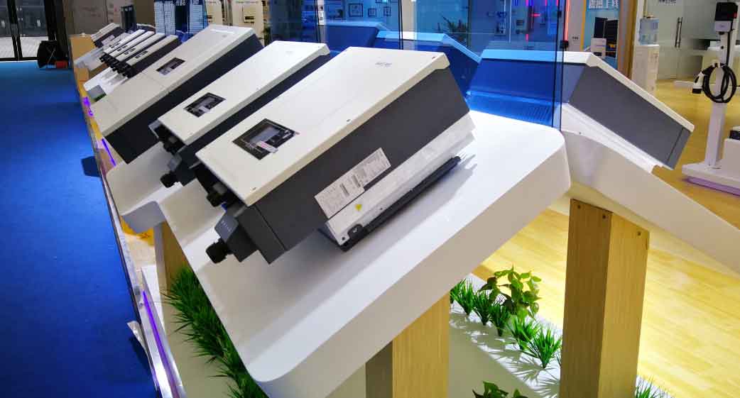
The image below illustrates a typical setup for energy storage inverters in solar applications, which is the target hardware for this control strategy.
2. Neutral-Point Voltage Balancing: The primary metric for my study was the difference between the two DC-link capacitor voltages, \( U_{C1} \) and \( U_{C2} \). During the initial 0-to-0.1-second period without active balancing, these voltages rapidly diverged due to the natural imbalance mechanism. The deviation peaked at approximately 60V. This is a severe imbalance that could damage switching devices and distort the output. At the 0.1-second mark, I activated the full MPC with the balancing cost function. The system response was immediate and effective. Within 0.022 seconds, the voltages converged to a stable and nearly equal state. The steady-state voltage difference was suppressed to within 4V, representing a 40% improvement over the unbalanced condition. This rapid convergence demonstrates the strong dynamic response of the proposed strategy, making it suitable for types of solar inverters that experience rapid changes in load or irradiation.
The simulation also showed robust performance under parameter disturbances, such as a sudden change in the capacitance value of one of the DC-link capacitors. The controller quickly adapted and restored the voltage balance, showcasing its inherent robustness and model-based predictive capabilities.
Conclusion
In this research, I have thoroughly investigated the single-phase NPC three-level inverter, focusing on the critical issue of neutral-point potential imbalance. I established that the core mechanism for this imbalance is the asymmetric charging of DC-link capacitors by small vectors, and I leveraged the opposite polarity of redundant small vectors as a control tool. To solve this problem, I developed and validated a novel multi-objective model predictive control strategy.
The proposed strategy integrates a cost function that simultaneously penalizes current tracking errors and neutral-point voltage deviations. By using the system model to predict future states, it autonomously selects the optimal switching state for each sampling period. The key advantages of this approach are:
- High Performance: It achieves both low THD (2.18%) in the output and fast neutral-point voltage balancing (within 0.022 seconds).
- Hardware Simplicity: The balancing is achieved without additional voltage sensors for the neutral point current, as the prediction model calculates these values.
- Robustness: The system maintains stability and performance even under parameter variations like changes in DC-link capacitance.
The simulation results confirm that this strategy is a highly effective solution for controlling types of solar inverters based on the NPC three-level topology. Looking ahead, this work has significant potential for practical implementation. Future research could explore extending this strategy to three-phase systems, optimizing the weighting factor \( \lambda \) online for variable operating conditions, and developing a hardware prototype for experimental validation. This MPC framework offers a powerful, flexible, and modern approach to mastering the control challenges in next-generation energy conversion systems, specifically for the wide variety of types of solar inverters used in industry today.