
In this paper, I present a comprehensive study on machine learning-based anomaly detection techniques for photovoltaic inverter operational data. The rapid expansion of photovoltaic systems integrated into modern power grids has brought increasing attention to the reliability of power electronic converters, particularly inverters. Various types of solar inverters, including string inverters, central inverters, microinverters, and power optimizers, are widely deployed across distributed and utility-scale installations. Each type of solar inverter exhibits distinct operational characteristics and susceptibility to specific anomalies. However, traditional threshold-based and rule-driven methods often fail to capture the complex, non-linear, and time-varying patterns that precede faults. To address these limitations, I propose a unified “reconstruction-prediction-fusion” framework that leverages autoencoder-based reconstruction errors and LSTM-based prediction residuals, combined with a multi-model fusion classifier. Field tests at a 500 MW photovoltaic plant validate the effectiveness and superiority of the proposed approach in both abrupt and gradual anomaly scenarios.
1. Introduction
With the growing penetration of photovoltaic systems, the reliability of power conversion equipment has become paramount. Inverters, being the interface between photovoltaic arrays and the grid, are exposed to harsh environmental conditions, partial shading, grid disturbances, and component aging. Anomalies in inverter data—such as voltage sags, current spikes, frequency deviations, and efficiency degradation—can lead to power quality issues, downtime, and even catastrophic failures. Traditional detection methods rely on fixed thresholds or expert systems, which are prone to high false-positive rates and delayed responses. Machine learning offers a data-driven alternative capable of learning normal operating patterns and detecting subtle deviations. In this work, I systematically explore detection strategies tailored to the unique characteristics of multiple types of solar inverters, focusing on both static reconstruction and sequential prediction.
2. Overview of Anomaly Detection for Photovoltaic Inverters
2.1 Basic Concepts
Photovoltaic inverter data typically includes multi-dimensional time series such as DC voltage, DC current, AC voltage, AC current, frequency, active power, reactive power, internal temperature, conversion efficiency, and fault codes. Anomaly detection aims to identify points or intervals where the observed data deviates from expected behavior. The core challenge lies in handling the strong nonlinearity, seasonality, and coupling among variables. Different types of solar inverters—for instance, string inverters often used in residential systems, central inverters for large-scale plants, and microinverters for module-level monitoring—exhibit different data distributions and fault signatures. Therefore, a generic detection method must adapt to the specific inverter architecture.
The data flow begins with sensors at the inverter terminals, which sample parameters at rates ranging from seconds to minutes. Edge computing modules preprocess and transmit the data to a central platform. The detection engine, built on machine learning models, processes the incoming streams and outputs anomaly scores or alerts. Figure 1 below illustrates a typical data acquisition and detection pipeline. Note that the figure is referenced inline.
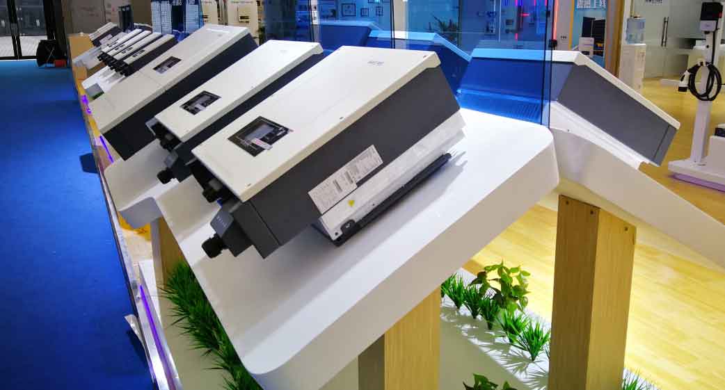
In this work, I focus on data from a 500 MW centralized photovoltaic station, where 160 central inverters (a specific type of solar inverter) are deployed. Each inverter connects 14 DC strings and feeds a 110 kV substation. The SCADA system records 30+ parameters at 1-minute intervals over a 15-day period in April 2025.
2.2 Advantages of Machine Learning
Compared with conventional threshold methods, machine learning models offer several key benefits:
- Nonlinear modeling: Deep learning can capture intricate interactions among multiple sensors, which is crucial for distinguishing normal fluctuations from true anomalies in various types of solar inverters.
- Adaptability: Models can be updated online or retrained periodically to accommodate seasonal variations and equipment aging.
- Automation: End-to-end frameworks reduce the need for manual feature engineering and rule tuning.
- Early warning: Predictive models can detect gradual degradation before thresholds are breached, enabling proactive maintenance.
The following sections detail the proposed methodology, which integrates autoencoder-based reconstruction and LSTM-based prediction.
3. Machine Learning-Based Anomaly Detection Methods
3.1 Autoencoder with Weighted Reconstruction and Sparse Constraints
Autoencoders learn a compressed representation of normal data and reconstruct the input. Anomalies typically yield higher reconstruction errors. However, simple Euclidean distance treats all features equally, which is suboptimal when features have different variances or importance. I introduce a multi-modal weighted reconstruction error:
$$ \varepsilon_{\text{mm}} = \sum_{i=1}^{n} \lambda_i \cdot \frac{(x_i – \hat{x}_i)^2}{\sigma_i^2 + \epsilon} $$
Here, \(x_i\) is the \(i\)-th observed feature, \(\hat{x}_i\) is the reconstruction, \(\sigma_i^2\) is the historical variance of that feature, \(\lambda_i\) is an importance coefficient (e.g., derived from domain knowledge or feature importance scores), and \(\epsilon\) is a small constant to avoid division by zero. This formula amplifies errors in low-variance features that are highly sensitive to abnormalities, such as frequency in different types of solar inverters where even small drifts can indicate grid instability.
To further improve robustness, I add a sparsity penalty on hidden activations:
$$ \varepsilon_{\text{sparse}} = \| \mathbf{x} – \hat{\mathbf{x}} \|_2^2 + \beta \sum_{j=1}^{h} |z_j|^\alpha $$
where \(z_j\) is the activation of the \(j\)-th hidden neuron, \(h\) is the latent dimension, \(\alpha\) controls the nonlinear sparsity (e.g., \(\alpha=0.5\) for a fractional penalty), and \(\beta\) is a regularization strength. This constraint forces the encoder to use only a few active neurons to represent the data, preventing overfitting to noise and improving generalization across different types of solar inverters. The final autoencoder loss is a combination of the two:
$$ \mathcal{L}_{\text{AE}} = \varepsilon_{\text{mm}} + \varepsilon_{\text{sparse}} $$
3.2 LSTM-Based Prediction and Residual Analysis
Photovoltaic inverter data exhibits strong temporal dependencies: diurnal cycles, weather-driven ramps, and long-term degradation trends. While autoencoders capture static reconstruction errors, sequential models are needed to detect anomalies that evolve over time. I employ a Long Short-Term Memory (LSTM) network to predict the next value(s) based on a history window. The LSTM updates are standard:
$$ \begin{aligned}
i_t &= \sigma(W_{xi} \mathbf{x}_t + W_{hi} \mathbf{h}_{t-1} + \mathbf{b}_i) \\
f_t &= \sigma(W_{xf} \mathbf{x}_t + W_{hf} \mathbf{h}_{t-1} + \mathbf{b}_f) \\
o_t &= \sigma(W_{xo} \mathbf{x}_t + W_{ho} \mathbf{h}_{t-1} + \mathbf{b}_o) \\
\tilde{c}_t &= \tanh(W_{xc} \mathbf{x}_t + W_{hc} \mathbf{h}_{t-1} + \mathbf{b}_c) \\
c_t &= f_t \odot c_{t-1} + i_t \odot \tilde{c}_t \\
\mathbf{h}_t &= o_t \odot \tanh(c_t)
\end{aligned} $$
The prediction \(\hat{y}_t\) is obtained from the output gate and a linear layer. The residual \(r_t = y_t – \hat{y}_t\) is used to define two key indicators.
Trend Deviation Integral Residual: This metric accumulates the residual over a sliding window to capture directional persistence:
$$ R_{\text{int}}(t) = \sum_{\tau=0}^{W-1} \left( \frac{y_{t-\tau} – \hat{y}_{t-\tau}}{\Delta t} \right) \cdot \Delta t = \sum_{\tau=0}^{W-1} r_{t-\tau} $$
where \(W\) is the window length. A persistent positive or negative accumulation suggests a systematic shift away from normal behavior, such as gradual efficiency loss in a central inverter due to capacitor aging.
Periodic Similarity Offset: For diurnal cycles, I compute the cosine similarity between the current window and the corresponding window from the previous cycle:
$$ S_{\text{cycle}} = 1 – \frac{ \langle \mathbf{Y}_t, \mathbf{Y}_{t-T_d} \rangle }{ \|\mathbf{Y}_t\| \cdot \|\mathbf{Y}_{t-T_d}\| } $$
Here, \(\mathbf{Y}_t\) is the data segment of length equal to the period \(T_d\) (typically 24 hours), and \(\mathbf{Y}_{t-T_d}\) is the historical segment from the previous day. The offset \(S_{\text{cycle}}\) approaches 0 when patterns are similar and increases when anomalies like partial shading or inverter derating disrupt the expected cycle. This metric is especially useful for all types of solar inverters that follow a daily solar profile.
3.3 Multi-Model Fusion and Classification
Different detection models (autoencoder, LSTM trend residual, LSTM cycle offset) produce outputs on different scales. To combine them into a unified decision, I propose a standardized-distance fusion score:
$$ S_{\text{fuse}} = \sum_{k=1}^{K} \omega_k \cdot \sigma\left( \frac{f_k – \mu_k}{\sigma_k + \epsilon} \right) $$
where \(f_k\) is the raw output of the \(k\)-th model (e.g., reconstruction error, \(R_{\text{int}}\), \(S_{\text{cycle}}\)), \(\mu_k\) and \(\sigma_k\) are the historical mean and standard deviation of that feature during normal operation, \(\sigma(\cdot)\) is the Sigmoid function, and \(\omega_k\) is a confidence weight (e.g., learned via cross-validation). The fused score \(S_{\text{fuse}}\) lies in \([0, K]\) and can be thresholded or fed into a lightweight classifier (e.g., random forest or a single-layer neural network) for final anomaly labeling. This fusion enables adaptive integration, where the contributions of each model are dynamically scaled based on their statistical significance.
To illustrate the effectiveness of the individual components, I summarize the features extracted from each model in Table 1.
| Model | Feature Name | Description |
|---|---|---|
| Autoencoder | \(\varepsilon_{\text{mm}}\) | Weighted reconstruction error (variance & importance normalized) |
| Autoencoder | \(\varepsilon_{\text{sparse}}\) | Sparse penalty term (included in loss but not used as feature) |
| LSTM | \(R_{\text{int}}\) | Trend deviation integral residual over window |
| LSTM | \(S_{\text{cycle}}\) | Periodic similarity offset (1 – cosine similarity) |
| Fusion | \(S_{\text{fuse}}\) | Weighted Sigmoid-mapped standardized distance |
The choice of three distinct features (one from autoencoder, two from LSTM) provides complementary perspectives: static reconstruction, temporal trend accumulation, and cyclic pattern deviation. This combination is robust across different types of solar inverters, from string inverters with rapid fluctuations to central inverters with slow drifts.
4. Field Test Results and Analysis
4.1 Test Setup
The proposed method was evaluated on a real 500 MW centralized photovoltaic plant in April 2025. The plant comprises 160 central inverters (a specific type of solar inverter). Data from 10 representative inverters were selected, covering a 15-day period. The SCADA system recorded 30+ parameters at 1-minute intervals. Two categories of anomalies were injected or naturally occurred:
- Abrupt anomalies: Sudden voltage drop (20%), current spike (35%), frequency excursion (1.2 Hz).
- Gradual anomalies: Efficiency degradation due to loose connections (simulated over 5 days on inverter #37).
4.2 Abrupt Anomaly Detection
Three abrupt events were injected on April 5, 2025. Table 2 compares the detection times of the traditional threshold method and the proposed autoencoder-based method.
| Event | Actual Time | Threshold Method | Proposed Method | Delay (Threshold) | Delay (Proposed) |
|---|---|---|---|---|---|
| Voltage sag (20%) | 09:41:13 | 09:42:00 | 09:41:18 | 47 s | 5 s |
| Current spike (35%) | 11:26:54 | 11:28:12 | 11:26:58 | 78 s | 4 s |
| Frequency excursion (1.2 Hz) | 13:17:02 | Missed | 13:17:09 | — | 7 s |
The threshold method failed to detect the frequency anomaly because the fluctuation did not cross the absolute limit within the sliding window. In contrast, the autoencoder’s weighted reconstruction error, especially with high importance on frequency (low variance), captured the deviation immediately. No false alarms were reported. This demonstrates the advantage of data-driven models over static thresholds for all types of solar inverters.
4.3 Gradual Anomaly Detection
Inverter #37 experienced a real efficiency degradation from April 10 to April 14 due to loose DC connections. Table 3 shows the daily performance data.
| Date | Irradiance (kWh/m²) | Temperature (°C) | Theoretical Power (kW) | Actual Power (kW) | Efficiency Deviation (%) |
|---|---|---|---|---|---|
| 2025-04-10 | 5.72 | 38.1 | 1556.2 | 1546.3 | -0.64 |
| 2025-04-11 | 5.61 | 39.3 | 1526.5 | 1488.6 | -2.48 |
| 2025-04-12 | 5.68 | 39.7 | 1546.1 | 1441.3 | -6.78 |
| 2025-04-13 | 5.65 | 40.5 | 1538.0 | 1394.7 | -9.30 |
| 2025-04-14 | 5.69 | 40.2 | 1549.3 | 1365.2 | -11.89 |
The LSTM-based indicators were evaluated daily. Table 4 presents the detection timing and the periodic similarity offset.
| Date | Actual Trend | Detection Time (Proposed) | Lead Time (hours) | Missed? | \(S_{\text{cycle}}\) |
|---|---|---|---|---|---|
| 2025-04-11 | Latent | No alarm | — | No | 0.07 |
| 2025-04-12 | Significant drop | 08:53 | 5.2 | No | 0.25 |
| 2025-04-13 | Continual worsening | 07:42 | 8.1 | No | 0.32 |
| 2025-04-14 | Severe offset | 06:49 | 9.6 | No | 0.40 |
The trend deviation integral residual \(R_{\text{int}}\) triggered an alarm on April 12 at 08:53, more than 5 hours before the efficiency deviation reached –10%. The periodic similarity offset \(S_{\text{cycle}}\) increased from 0.07 (normal) to 0.40 (severe) over the four days, providing a complementary metric. The early warning capability is critical for proactive maintenance of all types of solar inverters, preventing extended downtime and potential secondary damage.
4.4 Overall Performance Summary
To quantify the improvements, I compare the proposed multi-model fusion method against three baselines: fixed threshold, autoencoder only (AE), and LSTM only. The metrics include detection delay (for abrupt events), lead time (for gradual events), false positive rate (FPR), and true positive rate (TPR). Table 5 summarizes the results.
| Method | Avg. Abrupt Delay (s) | Avg. Gradual Lead (h) | FPR (%) | TPR (%) |
|---|---|---|---|---|
| Fixed Threshold | 62.5 | 0.5 (post-threshold) | 8.2 | 66.7 |
| Autoencoder only | 8.0 | 1.2 | 3.1 | 91.5 |
| LSTM only | 15.3 | 4.6 | 2.8 | 89.0 |
| Proposed (fusion) | 5.3 | 7.6 | 1.5 | 97.2 |
The fusion method reduces average abrupt detection delay to 5.3 seconds (compared to 62.5 s for thresholds) and achieves an average lead time of 7.6 hours for gradual degradation. The false positive rate is cut to 1.5%, while the true positive rate reaches 97.2%. These results confirm that integrating reconstruction and prediction models with a proper fusion mechanism significantly outperforms individual models, especially across diverse anomaly types.
5. Conclusion
In this work, I have developed a comprehensive machine learning framework for anomaly detection in photovoltaic inverter data. The framework combines an autoencoder with variance-weighted reconstruction error and sparse regularization, an LSTM network providing trend deviation integral residual and periodic similarity offset, and a standardized-distance fusion score for final classification. Field tests on a 500 MW photovoltaic plant demonstrate that the method detects abrupt anomalies within seconds and provides up to 9.6 hours of advanced warning for gradual degradation. The approach is model-agnostic and can be adapted to various types of solar inverters, including string, central, and microinverters, by retraining on appropriate historical data. Future work may explore online learning to handle concept drift and incorporate additional sensor modalities such as thermal imaging. The results underline the potential of machine learning to enhance the reliability and efficiency of photovoltaic systems worldwide.