
In this work, we investigate the influence of different state‑of‑charge (SOC) intervals on the capacity degradation and power scheduling of battery energy storage systems (BESS). Taking the minimum total cost of a hybrid power supply system as the optimization objective, we develop an operation optimization model for a multi‑battery energy storage system based on SOC interval division. The model is formulated as a mixed‑integer nonlinear programming (MINLP) problem. By solving this model, the optimal power scheduling strategy for the hybrid system is obtained. A case study of a photovoltaic (PV)‑BESS hybrid system is employed to demonstrate the effectiveness of the proposed method. Our results show that: (1) Compared with the full‑interval operation, a multi‑battery energy storage system operating in divided SOC intervals can substantially reduce the total cost of the hybrid power supply system—by 21.45% in the example. (2) The number of SOC operation intervals is not simply the more the better; it must be determined by a trade‑off between the operation and maintenance costs and the capacity degradation cost of battery energy storage units in a specific application scenario.
1. Introduction
In modern power systems, battery energy storage systems (BESS) play a crucial role in balancing supply and demand, smoothing the intermittency of renewable energy sources such as photovoltaic (PV) and wind power, and improving overall system reliability. However, the capacity degradation of batteries during cycling significantly affects their performance and economic viability. Numerous studies have shown that capacity fade is not only influenced by cycle number, depth of discharge, and temperature but also strongly depends on the SOC window in which the battery operates. For example, researchers have observed that batteries cycled at high SOC ranges degrade much faster than those cycled at low or medium SOC ranges. This difference suggests that by dividing the overall SOC operating range into multiple intervals and assigning different batteries to each interval, the overall degradation rate of the BESS can be reduced, leading to longer lifetime and lower total cost.
Motivated by these observations, we propose a novel operation optimization framework for multi‑BESS that explicitly considers the different capacity degradation characteristics of batteries operating in distinct SOC intervals. In our model, the BESS is composed of multiple battery units, each designated to operate within a specific SOC interval (e.g., low, medium, high, or full range). The entire hybrid system includes a PV generator, these battery units, the grid, and the load. The goal is to minimize the total annual cost, which comprises battery degradation cost and operation & maintenance cost, while satisfying power balance and battery operational constraints.
The remainder of this paper is organized as follows: Section 2 describes the problem in detail. Section 3 presents the mathematical optimization model. Section 4 provides a case study with real data to illustrate the approach. Section 5 discusses the economic impact of different SOC interval compositions. Section 6 concludes the paper.
2. Problem Description
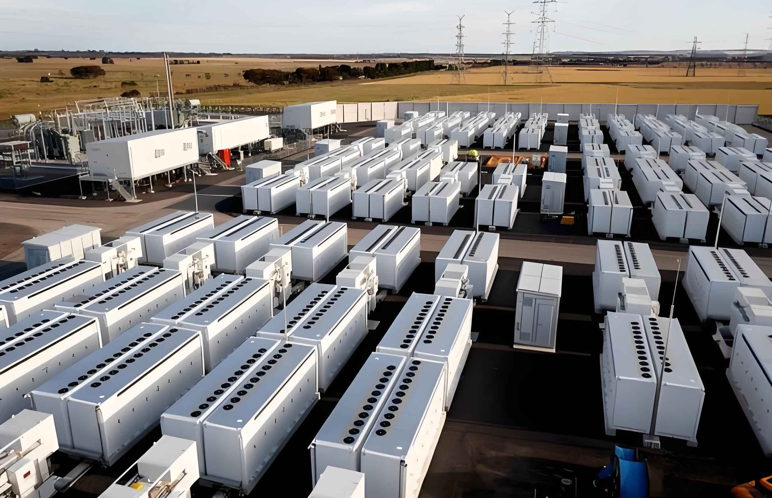
Figure 1 shows the conceptual diagram of the studied hybrid power supply system. The system consists of a PV generator, a multi‑battery energy storage system composed of \(n\) battery units operating in different SOC intervals, the electrical grid, and a load. The PV power can be used to serve the load, charge the batteries, or be sold to the grid. The batteries can discharge to the load when needed. The grid acts as a backup and also allows for power trading.
The problem is formally stated as follows:
- Given: Profile of PV power generation (hourly resolution), profile of user electricity demand, composition and capacity configuration of the multi‑BESS, and economic parameters (electricity price, battery unit cost, etc.).
- Determine: Optimal power scheduling for each component over the entire year (hourly time steps) to minimize the total annual cost.
- Constraints: Power balance, battery energy balance, SOC limits, charging/discharging power limits, and state‑of‑health (SOH) constraints.
We define two sets: \(\mathcal{N} = \{ n \,|\, n \text{ is a battery unit with a specific SOC interval}, n=1,2,\dots,N \}\) and \(\mathcal{K} = \{ k \,|\, k \text{ is a time interval (hour)}, k=1,2,\dots,K \}\). The planning horizon is one year with hourly resolution, so \(K = 8760\).
3. Optimization Model
3.1 Objective Function
The total annual cost \(C_{\text{total}}\) is minimized:
\[
\min \; C_{\text{total}} = C_{\text{bat}} + C_{\text{oper}},
\]
where \(C_{\text{bat}}\) is the battery degradation cost, representing the implicit cost due to capacity loss over the year, and \(C_{\text{oper}}\) is the operation and maintenance (O&M) cost, which includes the cost of running the batteries minus the revenue from selling electricity to the grid.
The battery degradation cost is computed as follows:
\[
C_{\text{bat}} = \sum_{n \in \mathcal{N}} \frac{1 – H_{n,K}}{H_{n,\text{ini}} – H_{n,\text{end}}} E_{n,\text{rated}} \, \mu_{n,b},
\]
with:
- \(H_{n,K}\): state‑of‑health of battery unit \(n\) at the end of the year (after \(K\) intervals);
- \(H_{n,\text{ini}}\): initial SOH (typically 1.0);
- \(H_{n,\text{end}}\): SOH at end of life (0.8 corresponds to 20% capacity loss);
- \(E_{n,\text{rated}}\): rated capacity of battery unit \(n\) (kWh);
- \(\mu_{n,b}\): unit cost of battery capacity (¥/kWh).
The O&M cost is given by:
\[
C_{\text{oper}} = \sum_{n \in \mathcal{N}} f_{n,\text{inv}} \, E_{n,\text{rated}} \, \mu_{n,b} – \sum_{k \in \mathcal{K}} \mu_{\text{sel}} \, E_{k,\text{OUT}},
\]
where \(f_{n,\text{inv}}\) is an operation cost coefficient for battery \(n\), \(\mu_{\text{sel}}\) is the selling price of electricity to the grid (¥/kWh), and \(E_{k,\text{OUT}}\) is the amount of electricity sold to the grid in interval \(k\) (kWh).
3.2 Constraints
3.2.1 Power Balance
PV generator balance:
\[
P_{k,S} \, t_k = P_{k,SD} \, t_k + \sum_{n \in \mathcal{N}} P_{n,k,SB} \, t_k + E_{k,\text{OUT}},
\]
where:
- \(P_{k,S}\): PV power output in interval \(k\) (kW);
- \(P_{k,SD}\): PV power directly supplied to load (kW);
- \(P_{n,k,SB}\): PV power charging battery unit \(n\) (kW);
- \(t_k\): duration of interval \(k\) (1 hour).
Load demand balance:
\[
P_{k,D} \, t_k = P_{k,SD} \, t_k + \sum_{n \in \mathcal{N}} P_{n,k,BD} \, t_k,
\]
where \(P_{k,D}\) is the load demand in interval \(k\) (kW), and \(P_{n,k,BD}\) is the discharge power from battery unit \(n\) to load (kW).
3.2.2 Battery Energy Balance
For each battery unit \(n\) and interval \(k\):
\[
E_{n,k,B} = E_{n,k-1,B} + \eta_{n,c} \, P_{n,k,SB} – \frac{P_{n,k,BD}}{\eta_{n,d}},
\]
where \(E_{n,k,B}\) is the stored energy (kWh) at the end of interval \(k\); \(\eta_{n,c}\) and \(\eta_{n,d}\) are charging and discharging efficiencies (both 0.95 in our case).
A cyclic condition over the entire year is enforced to ensure consistency:
\[
E_{n,0} = E_{n,K}.
\]
3.2.3 Capacity Degradation and SOH Model
The capacity fade per cycle follows a power‑law relationship with the number of equivalent cycles:
\[
D_{n,k} = A_n \left( \frac{x_{n,k}}{100} \right)^{b_n},
\]
where \(D_{n,k}\) is the capacity loss fraction in interval \(k\), and \(x_{n,k}\) is the number of equivalent full cycles during that interval, computed as:
\[
x_{n,k} = \frac{ \eta_{n,c} P_{n,k,SB} + \frac{P_{n,k,BD}}{\eta_{n,d}} }{ 2 E_{n,\text{rated}} } \, t_k.
\]
The factor 2 accounts for one full cycle (charge + discharge).
The coefficient \(A_n\) depends on the mean SOC \(S_{n,m}\) and the SOC window width \(\Delta S_n\) according to Saxena et al. (2016):
\[
A_n = A_{1,n} \, S_{n,m} \, (1 + A_{2,n} \, \Delta S_n + A_{3,n} \, \Delta S_n^2).
\]
Substituting into the degradation formula yields:
\[
D_{n,k} = A_{1,n} \, S_{n,m} \, (1 + A_{2,n} \, \Delta S_n + A_{3,n} \, \Delta S_n^2) \left( \frac{x_{n,k}}{100} \right)^{b_n}.
\]
The SOH is then defined as:
\[
H_{n,k} = 1 – D_{n,k}.
\]
The battery must maintain SOH above the end‑of‑life threshold during the planning period:
\[
0.8 \le H_{n,k} \le 1.0.
\]
3.2.4 SOC Constraints
The SOC \(S_{n,k}\) is:
\[
S_{n,k} = \frac{E_{n,k,B}}{E_{n,\text{rated}}}.
\]
Each battery unit has its own allowable SOC range:
\[
S_{n,\text{min}} \le S_{n,k} \le S_{n,\text{max}}.
\]
3.2.5 Charging/Discharging Binary and Power Limits
A binary variable \(z_{k,c}\) indicates the system‑wide charging mode (1 for charging, 0 for discharging). However, in a multi‑BESS, it is assumed that at any given time, all batteries operate in the same mode (all charging or all discharging) to simplify the model. The constraints are:
\[
0 \le \sum_{n \in \mathcal{N}} P_{n,k,SB} \le z_{k,c} \, P_{n,\text{rated}},
\]
\[
0 \le \sum_{n \in \mathcal{N}} P_{n,k,BD} \le (1 – z_{k,c}) \, P_{n,\text{rated}}.
\]
Individual battery power limits are:
\[
P_{n,k,SB} \, t_k \le \min \left( P_{n,\text{rated}}, (S_{n,\text{max}} – S_{n,\text{min}}) E_{n,\text{rated}} \right),
\]
\[
P_{n,k,BD} \, t_k \le \min \left( P_{n,\text{rated}}, (S_{n,\text{max}} – S_{n,\text{min}}) E_{n,\text{rated}} \right).
\]
3.2.6 Model Structure
The complete model is a mixed‑integer nonlinear programming (MINLP) problem. The variables and feasible domain are summarized as:
\[
J = \left\{ C_{\text{total}}, C_{\text{bat}}, C_{\text{oper}}, P_{k,SD}, P_{n,k,SB}, P_{n,k,BD}, E_{k,\text{OUT}}, E_{n,k,B}, S_{n,k}, D_{n,k}, H_{n,k}, x_{n,k}, z_{k,c} \right\},
\]
\[
D = \left\{ Y \,|\, \text{Eq. (1)–(19) hold} \right\}.
\]
We solve the model using the GAMS platform with the SCIP global solver (relative tolerance 5%).
4. Case Study
4.1 Data Description
The typical daily profiles of PV power and load demand are shown in Figure 2 (not reproduced here). The battery technology is ternary lithium‑manganese‑cobalt oxide (NMC). Four types of battery units are considered based on their SOC interval:
- L (Low): SOC ∈ [0, 0.2]
- M (Medium): SOC ∈ [0.2, 0.6]
- H (High): SOC ∈ [0.6, 1.0]
- T (Total): SOC ∈ [0, 1.0] (full interval)
Charging/discharging efficiency is 0.95. Rated power is one‑third of the rated capacity. The unit capacity cost is 1595.6 ¥/kWh. The operation cost coefficient \(f_{n,\text{inv}} = 0.01\). The selling price to the grid is set at a typical feed‑in tariff. The planning horizon is one year with hourly intervals.
Cycle life test data for the four battery types are taken from the literature (Zhu et al., 2017). Table 1 shows the remaining capacity (in %) as a function of cycle number for each SOC interval.
| Cycle Number | L (0–0.2) | M (0.2–0.6) | H (0.6–1.0) | T (0–1.0) |
|---|---|---|---|---|
| 0 | 100.00 | 100.00 | 100.00 | 100.00 |
| 100 | 98.73 | 97.01 | 95.02 | 96.16 |
| 200 | 95.86 | 93.98 | 92.94 | 92.32 |
| 300 | 94.36 | 92.02 | 89.30 | 89.63 |
| 400 | 93.05 | 89.87 | 86.16 | 84.78 |
| 500 | 91.92 | 87.07 | 80.48 | 71.82 |
| 600 | 90.87 | 82.66 | 68.72 | 50.23 |
Using these data, we fit the capacity degradation model (Equation 11) to obtain the parameters \(A_{1,n}\), \(A_{2,n}\), \(A_{3,n}\), and \(b_n\) for L, M, H batteries. Table 2 lists the fitted parameters with R² values above 0.95.
| Battery Type | Mean SOC \(S_{n,m}\) | Interval Width \(\Delta S_n\) | \(A_{1,n}\) | \(A_{2,n}\) | \(A_{3,n}\) | \(b_n\) | R² |
|---|---|---|---|---|---|---|---|
| L | 0.1 | 0.2 | 4.11858 | 10.84936 | 50.24678 | 0.82851 | 0.98 |
| M | 0.4 | 0.4 | 1.80043 | 3.60227 | 7.51058 | 1.02531 | 0.99 |
| H | 0.8 | 0.4 | 1.21842 | 1.60217 | 2.50542 | 1.49401 | 0.96 |
4.2 Results for B‑LMH vs. B‑T
We compare a multi‑BESS composed of L, M, and H units (denoted B‑LMH) with a single‑BESS using only the full‑interval T unit (B‑T). Each unit has a rated capacity of 500 kWh. The optimization results are given in Table 3.
| BESS Configuration | Unit | Degradation Rate (%) | Battery Degradation Cost (¥) | O&M Cost (¥) | Total Cost (¥) |
|---|---|---|---|---|---|
| B‑LMH | L | 1.6 | 305902.9 | ||
| M | 3.8 | ||||
| H | 1.6 | ||||
| Total | — | 281311.5 | 24591.5 | ||
| B‑T | T | 8.8 | 381500.0 | 7932.2 | 389432.2 |
| Total | — |
The total cost of B‑LMH is 305,902.9 ¥, which is 21.45% lower than that of B‑T (389,432.2 ¥). The primary reason is the much lower degradation cost in B‑LMH (281,311.5 ¥ vs. 381,500.0 ¥). The O&M cost of B‑LMH is higher (24,591.5 ¥ vs. 7,932.2 ¥), but this increase is far outweighed by the savings in degradation cost. This demonstrates that dividing the SOC operating range reduces overall capacity degradation, thus extending battery lifetime and lowering total cost.
4.3 Power Scheduling and SOC Profiles
We show the hourly power scheduling of the three battery units in B‑LMH (Figure 3) and the corresponding SOC variations. The charging power is plotted as positive, discharging as negative. It is observed that:
- The M‑unit is dispatched most intensively, followed by H and L. The ratio of total energy throughput among L:M:H is approximately 1.00:1.99:1.21, while the usable capacity ratio is 1.00:2.00:2.00. This indicates that the dispatch priority is L > M > H, because L has the lowest degradation rate, M has a moderate rate, and H has the highest.
- The SOC of each unit stays within its designated interval: L in [0,0.2], M in [0.2,0.6], H in [0.6,0.84]. The full‑interval T unit (B‑T) has SOC varying from 0.05 to 0.98.
4.4 Capacity Degradation Over Time
Figure 5 (in the original paper) shows the cumulative capacity loss and the capacity fade rate for each unit. Key observations:
- The M‑unit experiences the highest cumulative loss, while L and H have similar lower losses.
- The fade rate (loss per cycle) trends show three phases: initially M > L > H, then M > H > L, finally H > M > L. This complex behavior affects the optimal dispatch over the year.
5. Influence of SOC Interval Composition
To further explore the economic impact, we optimize the system for all possible combinations of battery units: single‑unit B‑L, B‑M, B‑H, B‑T; two‑unit B‑LM, B‑LH, B‑MH; and three‑unit B‑LMH. Table 4 lists the total cost and its components for each configuration.
| BESS Composition | Total Cost (¥) | Degradation Cost (¥) | O&M Cost (¥) | Unit Degradation Rates (%) |
|---|---|---|---|---|
| B‑T | 389,432.2 | 381,500.8 | 7,932.2 | 8.8 |
| B‑L | 319,960.9 | 280,924.0 | 39,036.9 | 1.4 |
| B‑M | 338,584.7 | 318,547.7 | 20,037.0 | 3.2 |
| B‑H | 286,356.0 | 264,432.8 | 156,159.0 | 2.7 |
| B‑LM | 326,291.1 | 299,916.1 | 26,375.0 | 1.6/2.9 |
| B‑LH | 287,719.3 | 260,085.7 | 27,633.7 | 1.6/2.3 |
| B‑MH | 307,883.1 | 286,903.0 | 20,980.1 | 3.8/1.9 |
| B‑LMH | 305,902.9 | 281,311.5 | 24,591.5 | 1.6/3.8/1.6 |
Key findings from Table 4:
- All configurations that use divided SOC intervals have lower total costs than the full‑interval B‑T. Even the worst divided configuration (B‑L) is better than B‑T.
- Among single‑unit systems, B‑H is the best (286,356.0 ¥), because its low degradation cost offsets its high O&M cost. B‑L and B‑M have higher degradation costs.
- Among two‑unit systems, B‑LH performs best (287,719.3 ¥), while B‑MH and B‑LM are worse. B‑LMH, with three units, gives a total cost of 305,902.9 ¥, which is higher than B‑LH. This indicates that adding more units does not always reduce cost; the optimal composition depends on the interplay between degradation and O&M costs.
These results highlight that the selection of SOC intervals and the number of battery units should be carefully optimized for each application. A larger number of intervals can reduce degradation but increases O&M cost (due to more units and control complexity). The trade‑off must be quantified using the proposed MINLP model.
6. Conclusions
In this work, we have presented a novel operation optimization framework for battery energy storage systems that exploits the different capacity degradation characteristics of batteries operating in distinct SOC intervals. By formulating a mixed‑integer nonlinear programming model and solving it for a PV‑BESS hybrid system, we have demonstrated the economic benefits of dividing the SOC operating range into several intervals and operating dedicated battery units in each interval. Our main conclusions are:
- Using a multi‑BESS with divided SOC intervals can significantly reduce the total annual cost compared to a single BESS operating over the full SOC range. In our case study, the cost reduction was 21.45%.
- The optimal number of SOC intervals is not unlimited. Adding more intervals increases complexity and O&M cost, while reducing degradation cost. The best composition is determined by the specific system parameters and cost structure. In our example, a combination of low‑ and high‑interval units (B‑LH) outperformed the triple‑interval system (B‑LMH).
- The proposed model provides a practical tool for designing and operating battery energy storage systems with enhanced lifetime and economic performance. Future work could extend the model to consider real‑time electricity prices, more detailed battery degradation models, and the possibility of using retired batteries in different SOC intervals.
We believe that the insights from this research can guide the deployment of battery energy storage systems in renewable‑rich power grids, leading to more sustainable and cost‑effective energy storage solutions.