
In the pursuit of optimizing the performance of photovoltaic systems, we have developed a methodology to accurately assess the degree of dust accumulation on solar panels. Dust buildup on solar panel surfaces is a critical factor that reduces energy output, and precise detection is essential for efficient maintenance. In our study, we first established a visual experimental platform for solar panel dust accumulation to quantify the relationship between dust density and image features. We introduced the concept of average grayscale value (MGV) to numerically represent the dust level. Subsequently, we employed five image fusion techniques on visible and infrared images captured from a dual-spectral imaging platform. By comparing the recognition performance of the resulting seven image types (visible, infrared, and five fused images), we identified that infrared images provide the most reliable and sensitive indicator of dust accumulation on solar panels, unaffected by varying irradiance conditions. This finding offers a robust theoretical basis for dust accumulation monitoring and is of significant importance for the maintenance of solar panel systems.
1. Experimental Systems
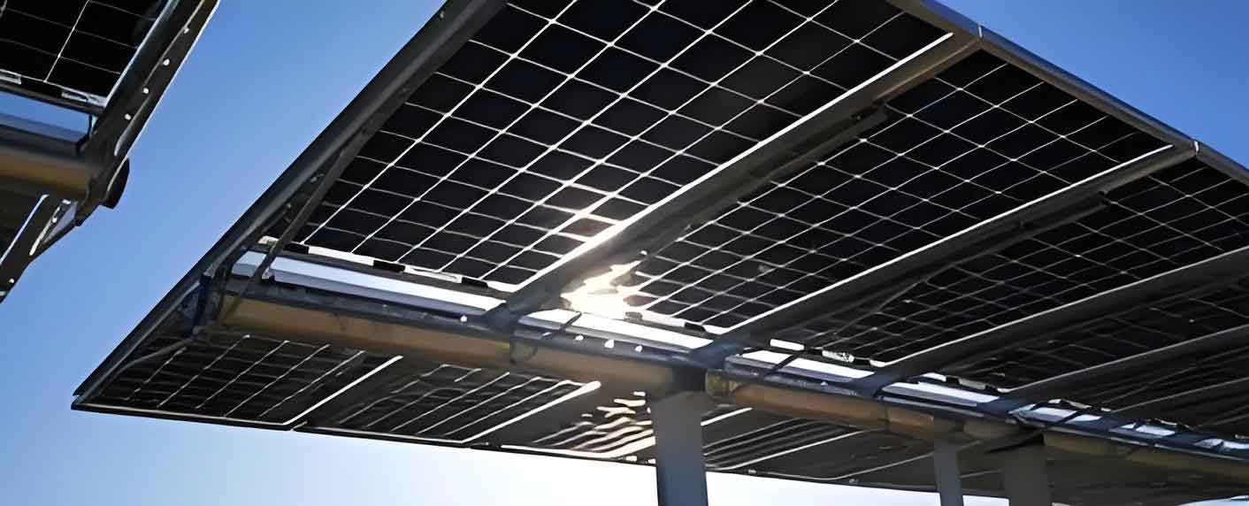
We constructed two distinct experimental setups to investigate dust accumulation on solar panels. The first setup, termed the solar panel dust visualization platform, was installed on the rooftop of a university building. It comprised multiple 50 W polycrystalline solar panels (dimensions 63 cm × 54 cm, active cell area 58 cm × 50 cm). The panels were allowed to accumulate dust naturally over time. We periodically collected the dust using a precise electronic balance (LQ-A20002, accuracy ±1 mg) and captured images before each collection using a Canon 3000D camera (18 MP effective pixels). The dust density was calculated as the collected dust mass divided by the panel area.
The second platform, a dual-spectral image fusion experimental platform, consisted of three YL285P-29b polycrystalline solar panels (285 W, dimensions 163 cm × 97 cm, active area 161 cm × 95 cm). One panel was cleaned daily (reference clean panel), one was cleaned every 15 days, and the third every 30 days (both considered dusty panels). A thermal imaging dual-spectral network camera (resolution 1920 × 1080, with RS485 transmission) captured both visible and infrared images. Visible images were taken at noon (12:00) after manual cleaning of the reference panel, while infrared images were captured at 23:00 on the same day to minimize effects of solar irradiance. The images were transmitted to a remote computer for analysis.
Key parameters of the solar panels and equipment are summarized in Tables 1 and 2.
| Parameter | Value |
|---|---|
| Dimensions (cm × cm) | 63 × 54 |
| Active cell area (cm × cm) | 58 × 50 |
| Open-circuit voltage (V) | 21.85 |
| Short-circuit current (A) | 2.85 |
| Operating voltage (V) | 18.20 |
| Operating current (A) | 2.70 |
| Maximum power (W) | 50 |
| Parameter | Value |
|---|---|
| Dimensions (cm × cm) | 163 × 97 |
| Active cell area (cm × cm) | 161 × 95 |
| Maximum power (W) | 285 |
| Open-circuit voltage (V) | 38.20 |
| Short-circuit current (A) | 9.55 |
| Operating voltage (V) | 31.50 |
| Operating current (A) | 9.05 |
2. Average Grayscale Value Calculation
2.1 Grayscale Conversion
We converted all captured color images to grayscale to simplify computation and highlight structural features. The weighted average method was applied:
$$ G_{\text{ray}} = 0.3 \times R + 0.59 \times G + 0.11 \times B $$
where $R$, $G$, $B$ are the red, green, and blue color channels, respectively, and $G_{\text{ray}}$ is the resulting grayscale value.
2.2 Perspective Transformation
To correct geometric distortion caused by non-orthogonal camera angles, we applied a perspective transformation. The general transformation is:
$$ \begin{bmatrix} X \\ Y \\ Z \end{bmatrix} = \begin{bmatrix} a_{11} & a_{12} & a_{13} \\ a_{21} & a_{22} & a_{23} \\ a_{31} & a_{32} & a_{33} \end{bmatrix} \begin{bmatrix} x \\ y \\ 1 \end{bmatrix} $$
After normalization ($Z’=1$), the mapping from original pixel $(x,y)$ to corrected coordinates $(X’,Y’)$ is:
$$ X’ = \frac{a_{11}x + a_{12}y + a_{13}}{a_{31}x + a_{32}y + 1},\quad Y’ = \frac{a_{21}x + a_{22}y + a_{23}}{a_{31}x + a_{32}y + 1} $$
We manually selected four control points on each region of interest (clean panel, two dusty panels) to compute the eight unknowns (setting $a_{33}=1$). The transformation aligns all panels to a common frontal view for fair comparison.
2.3 Grayscale Histogram and Average Grayscale Value
The grayscale histogram describes the frequency distribution of pixel intensities. Let $n_k$ be the number of pixels with grayscale value $k$ ($k=0,\dots,255$) and $n$ the total pixel count. The frequency $P(k)$ satisfies $\sum_{k=0}^{255} P(k)=1$. However, the histograms alone did not clearly differentiate dust levels. Therefore, we introduced the average grayscale value (MGV) as a single numerical metric:
$$ MGV = \frac{\sum_{i=0}^{255} i \cdot n_i}{n} $$
where $i$ is the grayscale value (0–255), $n_i$ the number of pixels with that value, and $n$ total pixels. A higher MGV indicates a brighter image, which we hypothesized correlates with less dust accumulation (since dust scatters light and reduces brightness).
2.4 Correlation Between MGV and Dust Density
We conducted 51 dust collection experiments from March 1 to April 20, 2023. Before each collection, we photographed the solar panel. After wiping the dust, drying, and weighing, we calculated the dust density. Figure 1 shows four representative images corresponding to different accumulation days (7, 14, 21, 28 days) with dust densities 0.39, 0.88, 1.18, 1.81 g/m² respectively. After grayscale conversion and perspective correction, we computed the MGV for each image. The relationship between dust density and MGV is shown in Figure 2.
Note: Figures are described in text; actual data points are plotted.
The plot (not shown here) reveals a clear monotonic increase in MGV with dust density. For example, a clean panel gave MGV~57.1, while a dusty panel after 28 days reached MGV~70.1. This validates that MGV can serve as a reliable proxy for dust accumulation on solar panels.
3. Image Fusion Methods
To evaluate the recognition performance under different imaging modalities, we applied five fusion algorithms to the visible and infrared images captured from the dual-spectral platform. All images had identical size $M \times N$. Let $A$ and $B$ be the visible and infrared images, respectively, and $F$ the fused image.
3.1 Max/Min Pixel Operation
For each pixel $(m,n)$:
$$ F(m,n) = \max\{A(m,n), B(m,n)\} \quad \text{or} \quad F(m,n) = \min\{A(m,n), B(m,n)\} $$
3.2 Pixel Averaging
$$ F(m,n) = \frac{A(m,n) + B(m,n)}{2} $$
3.3 Region Energy (Max/Min)
We compute the local energy around pixel $(i,j)$ using a 3×3 window with weight $w(p,q)$:
$$ E_A(i,j) = \sum_{p=-1}^{1} \sum_{q=-1}^{1} w(p,q) \cdot L_{A,N}(i+p,\,j+q) $$
where $L_{A,N}$ is the $N$-th layer of the Laplacian pyramid of image $A$. The fused pixel is selected from the image with higher (or lower) energy. We implemented both “region-energy max” and “region-energy min” approaches.
4. Recognition Performance Comparison
We collected 26 pairs of visible and infrared images over the period February 13 to March 10, 2023. All images were processed to extract three regions: left clean panel, middle dusty panel (cleaned every 15 days), and right dusty panel (cleaned every 30 days). For each of the seven image variants—visible, infrared, max-fusion, min-fusion, average-fusion, region-energy-max fusion, and region-energy-min fusion—we computed the MGV of each region. The MGV of the clean panel remained nearly constant over time, confirming its role as a baseline. The middle panel showed a drop in MGV after cleaning on March 1, then gradual increase. The right panel (never cleaned during the period) showed a continuous increase in MGV.
To quantify the sensitivity to dust, we defined the MGV difference $\Delta MGV = MGV_{\text{dusty}} – MGV_{\text{clean}}$ for each day. Figure 3 (not shown) plots these differences for the right (continuously dirty) panel. We performed linear regression on each time series and evaluated the goodness-of-fit using $R^2$:
$$ R^2 = 1 – \frac{\sum_{i=1}^{n} (y_i – \hat{y}_i)^2}{\sum_{i=1}^{n} (y_i – \bar{y})^2} $$
where $y_i$ is the actual $\Delta MGV$, $\hat{y}_i$ the predicted value from the linear fit, and $\bar{y}$ the mean of all $y_i$. The results are summarized in Table 3.
| Image Type | $R^2$ |
|---|---|
| Visible | 0.914 |
| Infrared | 0.964 |
| Max-pixel fusion | 0.935 |
| Min-pixel fusion | 0.932 |
| Average-pixel fusion | 0.928 |
| Region-energy max fusion | 0.937 |
| Region-energy min fusion | 0.935 |
The infrared image achieved the highest $R^2$ (0.964), indicating the most consistent linear trend with time, i.e., the least scatter and the strongest relationship between dust accumulation and MGV change. Moreover, the slope of the linear fit for infrared was the steepest among all seven types (not shown in table), meaning that the infrared images showed the most pronounced change in MGV as dust accumulated. This demonstrates that infrared imaging is the most robust method for detecting dust levels on solar panels, unaffected by variable daylight illumination.
5. Discussion and Conclusion
Our experiments confirm a clear correspondence between dust density on solar panels and the average grayscale value of their images. This relationship allows us to use MGV as a proxy for dust accumulation. Among the seven image types tested, infrared images outperformed both visible images and all five fusion images in terms of recognition accuracy (highest $R^2$) and sensitivity (largest slope). This superiority is attributed to the insensitivity of infrared imaging to ambient light variations, which often plague visible-light methods. The fusion methods, while improving over visible alone, still could not match the performance of pure infrared.
In practical applications, deploying an infrared camera on solar panel monitoring systems can provide reliable, real-time assessment of dust accumulation, facilitating timely cleaning and maintaining optimal energy generation. Future work could explore deep learning models trained on infrared image features to further automate the classification of dust levels.
In summary, we have introduced a quantitative approach to identifying dust accumulation on solar panels using average grayscale value, and we have demonstrated through comparative analysis that infrared imaging yields the best recognition performance. This finding provides a valuable theoretical foundation for dust monitoring in photovoltaic plants and emphasizes the importance of selecting appropriate imaging modalities for solar panel health assessment.