
The rapid integration of renewable energy sources such as wind and solar power into modern power grids has introduced significant operational challenges, primarily due to their inherent intermittency and unpredictability. To ensure grid stability and reliability, new energy storage systems play a crucial role by buffering the fluctuations and enabling time‑shifting of electricity supply. However, the scheduling of these energy storage systems is a complex multi‑objective optimization problem, affected by real‑time state‑of‑charge variations, market price signals, and operational constraints. Traditional methods often neglect dynamic battery conditions or fail to balance economic efficiency and scheduling accuracy. To address these limitations, we propose a novel scheduling optimization approach based on the fireworks algorithm, which excels in exploring complex, non‑linear search spaces. Our method integrates real‑time state‑of‑charge analysis into a bilevel optimization framework, aiming to maximize profit while minimizing scheduling deviations. Extensive simulations demonstrate that our approach significantly improves the stability, average charging/discharging power, and energy output of the energy storage system compared to existing techniques.
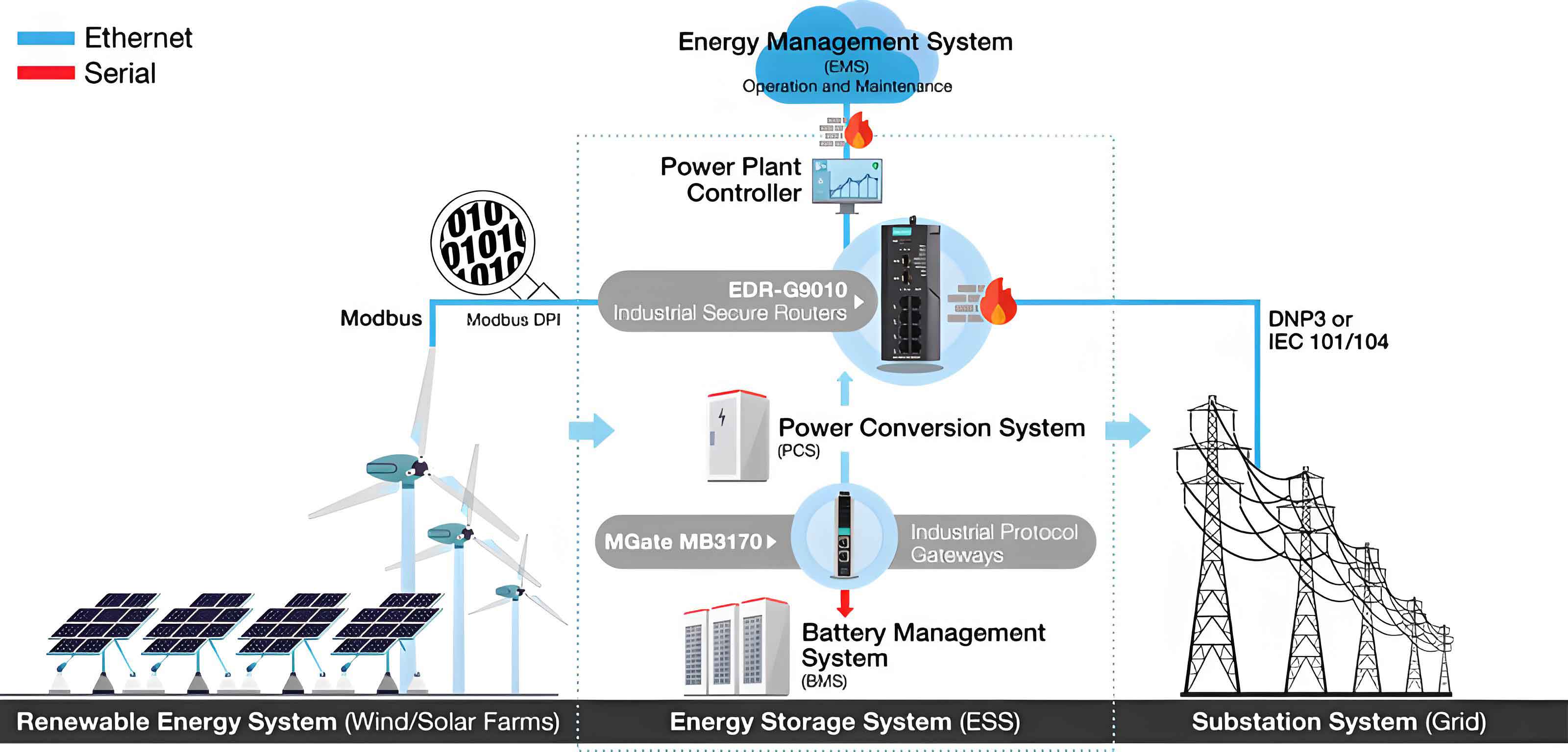
To effectively capture the dynamic behavior of an energy storage system, we first model its real‑time state of charge (SoC). A precise SoC estimation is essential because any misjudgment of the battery’s current capacity can lead to inappropriate charging/discharging decisions, thereby reducing the energy storage system’s lifespan and operational efficiency. The evolution of SoC over time is described by the following discrete equation:
$$
C_{\text{soc,bat,cap}}(t) = (1 – \rho) C_{\text{soc,bat,cap}}(t – 1) + \frac{\lambda P_{\text{bat,cap}} \Delta t \eta}{E_{\text{bat,cap}}}
$$
In this equation, $C_{\text{soc,bat,cap}}(t)$ denotes the state of charge at time $t$, $\rho$ is the self‑discharge rate, $P_{\text{bat,cap}}$ is the charging/discharging power, $\Delta t$ is the time interval, $\eta$ represents the efficiency, and $\lambda$ indicates the operational status (charging or discharging). $E_{\text{bat,cap}}$ is the total capacity of the energy storage system. To prevent deep discharging or overcharging, which can degrade the battery life, we impose lower and upper bounds on the SoC as follows:
$$
\begin{aligned}
C_{\text{soc,cap,min}} &\leq C_{\text{soc,cap}} \leq C_{\text{soc,cap,max}} \\
C_{\text{soc,bat,min}} &\leq C_{\text{soc,bat}} \leq C_{\text{soc,bat,max}}
\end{aligned}
$$
By incorporating these real‑time SoC constraints into the scheduling model, the energy storage system can make more informed decisions that respect the physical limits of the battery, thereby ensuring both longevity and safety. This forms the foundation for the subsequent bilevel optimization framework.
We formulate the scheduling problem as a bilevel optimization model. The upper level addresses the overall dispatch of the energy storage system, while the lower level coordinates the system’s flexible resources to meet the dispatch commands accurately. The two levels are coupled through the scheduled power output and the actual response, ensuring minimal discrepancy.
Upper‑level model: The upper level aims to achieve two primary objectives: maximizing the profit of the energy storage system and minimizing the scheduling deviation.
The profit maximization objective accounts for the total revenue from energy trading minus the operational costs of all generation units, including wind, photovoltaic (PV), hydropower, conventional generators, and the energy storage system itself. It is expressed as minimizing the normalized cost:
$$
\min f_{11} = \frac{1}{C_H – (C_V + C_Y + C_G + C_W + C_S + C_R)}
$$
Here, $C_H$ represents the revenue from interconnection transactions, and $C_V$, $C_Y$, $C_G$, $C_W$, $C_S$, $C_R$ denote the operational costs of various units. Simultaneously, we seek to minimize the absolute deviation between the scheduled power $P_Q^t$ and the actual power $P_Q^{+t}$ returned from the lower level:
$$
\min f_{12} = \sum_{t=1}^{T} |P_Q^t – P_Q^{+t}|
$$
These two objectives are combined into a single weighted sum (with appropriate normalization) to form the upper‑level optimization.
Lower‑level model: The lower level allocates the dispatch tasks to controllable loads, such as curtailable and shiftable loads, while respecting the operational constraints of the energy storage system. The objective is to minimize the system’s cost and ensure the best economic benefit. The cost includes compensation for curtailed load and shifted load:
$$
\min f_{21} = \sum_{t=1}^{T} \left( \xi_{KL} \cdot y_{KL}^t \cdot P_{KL} + \xi_{BL} \cdot |P_{BL}| \right)
$$
where $\xi_{KL}$ and $\xi_{BL}$ are price indices, $y_{KL}^t$ is the binary status of curtailment, $P_{KL}$ is curtailed power, and $P_{BL}$ is shifted power. Additionally, we aim to minimize the percentage of load curtailment and shifting, which also reflects the social welfare objective:
$$
\min f_{22} = 1 – \lambda_{KL} \cdot \frac{P_{KL}}{P_{KL}^{\max}} + 0.5 \cdot \lambda_{BL} \cdot \frac{P_{BL}}{P_{BL}^{\max}}
$$
By solving the lower‑level model, the scheduling deviations are minimized, and the overall economic efficiency of the energy storage system is maximized.
To solve the above bilevel optimization problem, we adopt the fireworks algorithm, a nature‑inspired metaheuristic known for its strong global search capability and adaptability to high‑dimensional, non‑linear problems. The algorithm mimics the explosion process of fireworks, where each firework generates multiple sparks within an explosion radius. The key steps are summarized below.
First, initialize the population of $N$ fireworks, their positions, and the mutation probability. Second, for each firework $i$, compute the number of sparks $Z_i$ and the explosion radius $D_i$ according to its fitness $f_i$:
$$
Z_i = N’ \cdot \frac{y_{\max} – f_i + \varepsilon}{\sum_{i=1}^{N} (y_{\max} – f_i) + \varepsilon}, \quad D_i = A \cdot \frac{f_i – y_{\min} + \varepsilon}{\sum_{i=1}^{N} (f_i – y_{\min}) + \varepsilon}
$$
Here, $y_{\max}$ and $y_{\min}$ are the maximum and minimum fitness values in the population, $\varepsilon$ is a small constant to avoid division by zero, $N’$ is the total number of sparks, and $A$ is the standard explosion radius. Sparks are generated randomly within the explosion radius, and a Gaussian mutation operator is applied to generate additional sparks for diversity. Then, a chaotic search mechanism is used to update the candidate population:
$$
M_{k}^{i+1} = 1 – 2 (M_{k}^{i})^2
$$
where $M_{k}^{i}$ is a chaotic variable in the interval $(-1, 1)$. After chaotic iterations, if a better solution is found, it replaces the original. Finally, a roulette‑wheel selection based on distance probabilities determines whether to terminate the global search. The selection probability for individual $i$ is:
$$
p_i = \frac{\sum_{j=1}^{K} d(N_i, N_j)}{\sum_{i=1}^{K} M_{k}^{i+1}}
$$
If $p_i$ falls within the acceptable range, the algorithm outputs the optimal solution; otherwise, it returns to the explosion step with increased iterations.
The proposed method was validated on a realistic test system comprising 26 thermal units (total capacity 3110 MW), a peak load of 2800 MW, a PV station of 700 MW, a battery energy storage system of 50 MW/80 MW·h (minimum stored energy 16 MW·h, charging/discharging efficiency 90%), and a pumped‑hydro storage unit (rated 300 MW, total reservoir 1500 MW·h). We compared our technique (denoted as “Proposed”) with two existing methods: a flow‑adaptive scheduling method (“Flow‑Adaptive”) and a multi‑energy storage scheduling method (“Multi‑Storage”). Three performance metrics were evaluated: stability of the energy storage system, average charging/discharging power, and energy output of the storage equipment.
Stability of the energy storage system: Stability was assessed by monitoring the battery’s state of charge (SoC) over different time intervals. The SoC variation under the proposed method remained within a narrow range, indicating a well‑balanced charge/discharge strategy that avoids deep cycles and reduces stress on the battery. In contrast, the other two methods exhibited larger fluctuations, suggesting less stable operation and potential degradation of the energy storage system. The following table summarizes the SoC range observed during the simulation period.
| Method | Minimum SoC (%) | Maximum SoC (%) | Standard Deviation |
|---|---|---|---|
| Proposed | 38.2 | 61.5 | 4.3 |
| Flow‑Adaptive | 22.7 | 78.9 | 12.8 |
| Multi‑Storage | 19.4 | 82.3 | 15.6 |
The results clearly show that the proposed method delivers the most stable SoC performance, which is crucial for the long‑term reliability of the energy storage system.
Average charging/discharging power: The average power during charging and discharging reflects the energy storage system’s ability to respond to grid requirements. Higher average power indicates more effective utilization of the storage capacity. The average charging/discharging power for each method is tabulated below.
| Method | Average Charging Power | Average Discharging Power |
|---|---|---|
| Proposed | 42.8 | 41.5 |
| Flow‑Adaptive | 35.2 | 34.1 |
| Multi‑Storage | 30.6 | 29.3 |
As seen, our method achieves the highest average power, meaning the energy storage system is better utilized to smooth renewable output and supply peak demand.
Energy output of the storage equipment: This metric measures the actual energy delivered by different generation sources after optimization. A higher output from renewable sources and a lower amount of transferred (wasted) energy indicate a more efficient scheduling scheme. The following table presents the energy generation from wind, PV, hydro, and the transferred storage energy.
| Source | Proposed | Flow‑Adaptive | Multi‑Storage |
|---|---|---|---|
| Wind | 1365.25 | 1125.12 | 1012.36 |
| PV | 856.26 | 652.32 | 567.59 |
| Hydro | 220.26 | 180.32 | 170.26 |
| Transferred energy | 128.36 | 250.36 | 365.21 |
The proposed method yields the highest renewable energy output (wind, PV, hydro) and the lowest amount of transferred energy, indicating that the scheduling algorithm effectively coordinates the energy storage system to match generation with load, minimizing curtailment and waste.
In conclusion, we have presented a novel scheduling optimization method for new energy storage systems based on the fireworks algorithm. By integrating real‑time state‑of‑charge analysis into a bilevel optimization framework, our approach simultaneously maximizes profit, minimizes scheduling deviations, and ensures stable operation. Experimental results on a realistic power system model demonstrate that the proposed method outperforms existing techniques in terms of SoC stability, average charging/discharging power, and renewable energy output. The fireworks algorithm’s strong global search ability effectively handles the complex, multi‑constraint nature of the energy storage system scheduling problem. Future work will extend the method to incorporate more renewable sources and grid‑scale uncertainties.