
In this study, we numerically investigated the heat transfer characteristics of parallel air‑cooled and liquid‑cooled battery modules designed for a 50 A·h lithium‑ion energy storage cell array. The objective is to quantitatively compare the cooling effectiveness, flow resistance, overall thermo‑hydraulic performance, and ambient temperature sensitivity between the two thermal management strategies. The insights derived here can guide the selection and optimization of cooling methods for large‑scale energy storage cell systems.
1. Introduction
Lithium‑ion energy storage cells are widely adopted in electric vehicles and grid‑scale energy storage due to their high energy density and long cycle life. However, these cells generate significant heat during charging and discharging, and elevated temperatures can lead to thermal runaway and capacity degradation. An effective thermal management system (TMS) is thus essential to maintain the energy storage cell temperature within a safe range (typically 15–35 °C). Among various TMS techniques, air cooling (forced convection) and liquid cooling (indirect liquid‑cold plate) are the most mature and commonly implemented. While air cooling offers simplicity and low cost, its heat transfer coefficient is limited; liquid cooling provides superior cooling performance but adds complexity and weight. The choice between them depends on specific application requirements such as heat load, allowable temperature difference, and environmental conditions.
In the present work, we built two three‑dimensional numerical models of a battery module containing 26 energy storage cells arranged in two parallel rows. The air‑cooled module features parallel flow channels with inlet/outlet plenums, while the liquid‑cooled module integrates cold plates with serpentine‑parallel channels. Using validated computational fluid dynamics (CFD) simulations, we systematically compared the modules under various cooling medium temperature rises (ΔTf) and ambient temperatures. The analysis focuses on: (i) heat transfer performance via maximum cell temperature (Tmax), temperature uniformity (ΔTc), and the dimensionless Colburn‑J factor; (ii) flow resistance characterized by pressure drop ΔP and friction factor F; (iii) overall thermo‑hydraulic performance evaluated by the θ = J/F factor; and (iv) sensitivity to ambient temperature variations.
2. Numerical Methodology
2.1 Geometry and Physical Model
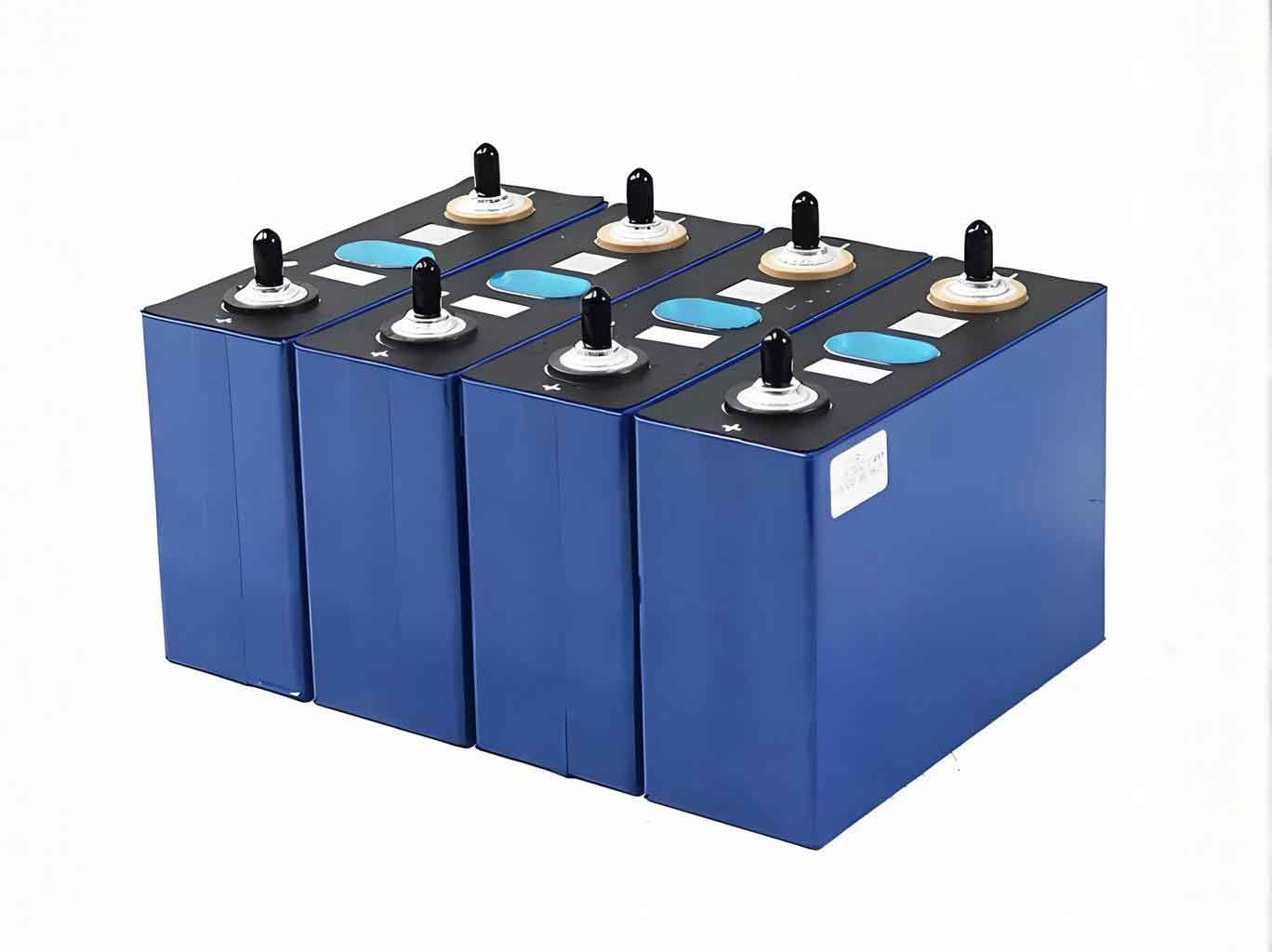
The battery module consists of 26 prismatic energy storage cells (dimensions 205 mm × 174 mm × 72 mm, nominal voltage 3.7 V, capacity 50 A·h). During constant‑current (1 C) charging, the total heat generation rate is 822.12 W (31.62 W per cell). The cells are arranged in two rows (A and B), each containing 13 cells. For air cooling, the module includes a lower diffuser plenum, parallel inter‑cell channels (width 10 mm), and an upper collector plenum. For liquid cooling, an aluminum cold plate with 3.5 mm thick parallel channels is placed in thermal contact with the cells via thermal pads (1.5 mm thick, thermal conductivity 2 W/(m·K)). The coolant is a 50% ethylene‑glycol/water mixture. All external surfaces except the cold plate bottom are assumed adiabatic.
2.2 Governing Equations and Turbulence Model
The simulations are based on the finite‑volume method with the following steady‑state governing equations:
Continuity:
$$
\nabla \cdot (\rho_f \mathbf{u}) = 0 (1)
$$
Momentum:
$$
\nabla \cdot (\rho_f \mathbf{u} \mathbf{u}) = -\nabla P + \mu \nabla^2 \mathbf{u} (2)
$$
Energy (fluid):
$$
\rho_f c_f \mathbf{u} \cdot \nabla T_f = \nabla \cdot (\lambda_f \nabla T_f) (3)
$$
Energy (solid cell, anisotropic):
$$
0 = \lambda_x \frac{\partial^2 T_b}{\partial x^2} + \lambda_y \frac{\partial^2 T_b}{\partial y^2} + \lambda_z \frac{\partial^2 T_b}{\partial z^2} + q_b (4)
$$
Turbulence is modeled via the standard k‑ε model with enhanced wall treatment. The SIMPLE algorithm is used for pressure‑velocity coupling, and first‑order upwind discretization is applied to momentum, turbulent kinetic energy, and dissipation rate. Convergence is declared when residuals are below 10⁻⁴ for continuity and momentum, and 10⁻⁶ for energy, and when monitored Tmax and ΔP change by less than 0.1%.
2.3 Material Properties and Boundary Conditions
The material properties used in the simulations are listed in Table 1. The ambient temperature is set to 20 °C unless otherwise stated. The inlet boundary is velocity‑inlet with a prescribed temperature of 20 °C; the outlet is pressure‑outlet (gauge pressure 0 Pa). The flow rates for both cooling methods are derived from the energy balance: \( q_b = Q \rho_f c_f \Delta T_f \), where ΔTf is the temperature rise of the cooling medium across the module. Table 2 summarizes the required flow rates for ΔTf = 1, 2, 4, 6, 8, 10 °C.
| Material | ρ (kg/m³) | μ (mPa·s) | cp (J/(kg·K)) | λx, λy, λz (W/(m·K)) |
|---|---|---|---|---|
| Air | 1.205 | 0.0183 | 1013 | 0.0267 |
| 50% EG/Water | 1071.1 | 3.94 | 3300 | 0.384 |
| Battery cell (anisotropic) | 2230 | – | 982 | λx=λz=23.88, λy=0.65 |
| Aluminum 6061 | 2680 | – | 947 | 156 |
| ΔTf (°C) | Air flow rate Qair (m³/h) | Liquid flow rate Qliquid (×10⁻³ m³/h) |
|---|---|---|
| 1 | 39.873 | 13.770 |
| 2 | 19.937 | 6.885 |
| 4 | 9.968 | 3.443 |
| 6 | 6.646 | 2.295 |
| 8 | 4.984 | 1.721 |
| 10 | 3.987 | 1.377 |
2.4 Mesh Independence Study
We performed a mesh sensitivity analysis using poly‑hexcore (polyhedral) grids with four prism layers near walls. For both the air‑cooled and liquid‑cooled models, five mesh sizes were tested (1.2 million to 8.5 million cells). The results for Tmax and ΔP stabilized when the mesh count reached approximately 5.6 million cells. Further refinement changed Tmax by less than 0.5% and ΔP by less than 1.6% for air cooling; for liquid cooling, the changes were less than 0.1% and 0.3%, respectively. Therefore, all subsequent simulations use a mesh of about 5.64 million cells with an average orthogonal quality >0.8 and skewness <0.15.
3. Results and Discussion
3.1 Heat Transfer Performance
Figure 1 compares the maximum cell temperature (Tmax), minimum temperature (Tmin), average temperature (Tave), and maximum temperature difference across cells (ΔTc) for both cooling methods under ΔTf = 1–10 °C. As ΔTf increases, all temperatures rise for both methods, but the rate of increase is more pronounced for air cooling. For ΔTf ≥ 2 °C, the liquid‑cooled module exhibits lower Tmax and Tmin, indicating superior thermal safety. However, at ΔTf = 1 °C, the air‑cooled module shows a Tmax that is 2.5 °C lower than the liquid‑cooled one, while Tmin values are similar. Thus, there is a crossover point for Tmax at ΔTf ≈ 1.76 °C (determined by interpolation). For ΔTc, the crossover occurs at ΔTf ≈ 3.15 °C. This means that when the required cooling medium temperature rise is very low, air cooling can actually provide better temperature uniformity and lower peak temperatures, but for typical practical designs (ΔTf > 3 °C), liquid cooling is clearly superior.
To further assess heat transfer quality, we use the Colburn‑J factor:
$$
J = \frac{Nu}{Re\,Pr^{1/3}} (5)
$$
For the present steady‑state condition, the total heat transfer rate is fixed by the cell heat generation, independent of ΔTf. The computed J values are: \( J_{air} = 2.91 \times 10^{-3} \) and \( J_{liquid} = 9.67 \times 10^{-3} \). Hence, the liquid‑cooled module has a heat transfer performance about 3.32 times higher than that of the air‑cooled module, primarily due to the much higher thermal conductivity and heat capacity of the coolant.
The temperature distribution within the module at ΔTf = 6 °C is illustrated in Figure 2 (using the cross‑section through the center of Row A). For air cooling, the cell temperatures exhibit a “rise‑plateau‑fall” pattern along the flow direction, directly correlated to the non‑uniform airflow distribution among the parallel channels. The cell‑to‑cell temperature difference ΔTc reaches 6.1 °C. In contrast, the liquid‑cooled module shows excellent temperature uniformity: ΔTc is only 0.5 °C across all cells, and the temperatures increase monotonically along the flow due to coolant heating, but the variation is very small (less than 1 °C). This demonstrates the inherent advantage of liquid cooling in maintaining uniform thermal conditions among individual energy storage cells.
We place the image link here (Figure 2 shows a representative temperature contour of the liquid‑cooled module):
3.2 Flow Resistance Performance
The pressure drop ΔP across the module is a critical indicator of pumping power requirement. Figure 3 shows ΔP as a function of ΔTf. As ΔTf increases (i.e., flow rate decreases), ΔP decreases nonlinearly for both methods. The liquid‑cooled module always exhibits a higher ΔP than the air‑cooled one, but the difference narrows at higher ΔTf. For instance, at ΔTf = 1 °C, ΔPliquid ≈ 7500 Pa vs. ΔPair ≈ 120 Pa; at ΔTf = 10 °C, ΔPliquid ≈ 400 Pa vs. ΔPair ≈ 15 Pa. The dominant flow resistance in both modules originates from the manifolds (diffuser/collector) and the turning/combining regions rather than the straight channels.
A dimensionless friction factor is defined as:
$$
F = \frac{2 \Delta P}{\rho_f u^2} (6)
$$
Figure 4 plots F for both cooling methods. The friction factor for liquid cooling is 5.2 to 17.6 times larger than that for air cooling over the studied ΔTf range. Moreover, F increases almost linearly with ΔTf for air cooling, but more steeply for liquid cooling. This indicates that liquid cooling is penalized more heavily at low flow rates (high ΔTf) in terms of relative friction.
3.3 Overall Thermo‑Hydraulic Performance
To balance heat transfer enhancement against pressure drop, we compute the overall performance factor:
$$
\theta = \frac{J}{F} (7)
$$
A higher θ means better heat transfer per unit flow resistance. The results are compiled in Table 3. Over the entire ΔTf range, the liquid‑cooled module achieves θ values 1.27 to 1.71 times those of the air‑cooled module. For example, at ΔTf = 1 °C, θliquid = 2.30 × 10⁻³ vs. θair = 1.34 × 10⁻³; at ΔTf = 10 °C, θliquid = 2.20 × 10⁻³ vs. θair = 1.72 × 10⁻³. Therefore, despite its higher flow resistance, liquid cooling offers a net benefit in thermo‑hydraulic efficiency, especially at higher flow rates (lower ΔTf). This advantage stems from the superior heat transfer capability of liquids.
| ΔTf (°C) | θair (×10⁻³) | θliquid (×10⁻³) | θliquid/θair |
|---|---|---|---|
| 1 | 1.34 | 2.30 | 1.72 |
| 2 | 1.95 | 2.77 | 1.42 |
| 4 | 2.59 | 3.47 | 1.34 |
| 6 | 3.05 | 3.86 | 1.27 |
| 8 | 3.50 | 4.20 | 1.20 |
| 10 | 4.40 | 4.40 | 1.00 |
3.4 Influence of Ambient Temperature
The sensitivity of the thermal management system to ambient temperature Te is critical for practical applications. We fixed ΔTf = 6 °C and varied Te from 0 °C to 30 °C. Figure 5 presents the resulting Tmax, Tmin, Tave, and ΔTc. For the air‑cooled module, raising Te from 0 °C to 30 °C increases Tmax by 4.25 °C, Tmin by 8.34 °C, and Tave by 5.17 °C, while ΔTc decreases by 4.10 °C. The large variation in Tmin and the drop in ΔTc indicate that air cooling is strongly affected by ambient conditions, mainly because the air temperature itself determines the cooling potential. In contrast, the liquid‑cooled module shows remarkable robustness: Tmax changes only by 1.06 °C, Tmin changes by 0.03 °C, Tave varies by 0.67 °C, and ΔTc changes by 1.03 °C. The liquid coolant effectively buffers against ambient fluctuations, making liquid cooling far more suitable for environments with wide temperature swings, such as outdoor energy storage cell cabinets.
4. Conclusions
This study provides a comprehensive numerical comparison between parallel‑flow air‑cooled and liquid‑cooled thermal management systems for a 26‑cell lithium‑ion energy storage cell module. The key findings are summarized as follows:
- Heat transfer performance: When evaluating Tmax and ΔTc, there exists a crossover point in the cooling medium temperature rise (ΔTf ≈ 1.76 °C for Tmax, ≈3.15 °C for ΔTc). Below this point, air cooling yields lower peak temperatures and better uniformity; above it, liquid cooling is superior. On the basis of the Colburn‑J factor, liquid cooling outperforms air cooling by a factor of 3.32.
- Flow resistance: The liquid‑cooled module exhibits higher pressure drop and friction factor F (5–18 times larger than air cooling). However, the major pressure losses occur in the manifold regions, suggesting that improved design of the inlet/outlet plenums could reduce pumping penalties for both methods.
- Overall thermo‑hydraulic performance: The composite θ = J/F factor demonstrates that liquid cooling is consistently more efficient than air cooling, with a performance ratio of 1.27–1.71 over the studied ΔTf range. The advantage is most pronounced at lower ΔTf (higher flow rates).
- Ambient temperature sensitivity: Liquid cooling exhibits excellent resilience to ambient temperature variations (0–30 °C), with Tmax changes of only 1.1 °C, whereas air cooling experiences a 4.3 °C rise in Tmax and an 8.3 °C rise in Tmin. Therefore, for energy storage cell systems operating in variable outdoor climates, liquid cooling is strongly recommended.
The methodology and results presented here can guide engineers in selecting an appropriate cooling strategy and in optimizing the geometry of parallel‑channel thermal management systems for large‑format energy storage cell modules.