
In series-connected energy storage systems, the inconsistency among individual energy storage cells is a persistent challenge that directly limits the usable capacity and operational efficiency of the entire system. Over time, factors such as manufacturing tolerances, self-discharge rate variations, and thermal gradients cause the voltage working ranges of energy storage cells to drift apart. This drift results in premature charge or discharge termination, reducing the effective throughput of the system. Accurate state-of-charge (SOC) estimation and effective balancing control are therefore critical for maximizing capacity utilization. Conventional passive balancing strategies, which rely on fixed voltage thresholds or offline SOC curves, often fail under real-world operating conditions due to the flat voltage plateau of lithium iron phosphate (LFP) chemistry and the progressive aging of energy storage cells. To address these limitations, we propose a novel balancing framework that integrates dynamic SOC calibration at the end of charge/discharge phases with a full-time adaptive balancing control algorithm. This strategy, referred to as the Self-Calibration Balance Strategy (SCBS), continuously updates the reference voltage–SOC relationship for each energy storage cell based on the actual operating data, identifies cells requiring equalization, and iteratively adjusts the balancing duration until the minimum-capacity energy storage cell achieves full utilization. In this paper, we describe the system topology, the mathematical model of SCBS, and the experimental validation conducted on three 200 kWh LFP energy storage cabinets operating under a typical two‑cycle daily profile. Detailed comparisons are made against the conventional minimum‑voltage balance strategy (MVBS) and the average‑voltage balance strategy (AVBS). The results demonstrate that SCBS achieves superior balancing efficiency and capacity recovery, with a 5.9% increase in discharge capacity over 12 days, outperforming AVBS by a factor of 4.9. Furthermore, we discuss the energy loss, thermal impact, long‑term stability, and scalability of the proposed approach for different cell types and module sizes.
System Architecture and Passive Balancing Circuit
The distributed energy storage system under study consists of 224 LFP energy storage cells connected in series, each with a nominal capacity of 280 Ah and a nominal voltage of 3.2 V. The entire system is rated at 200 kWh and operates at a nominal DC bus voltage of 716.8 V. A passive balancing circuit employing shunt resistors is integrated into the battery management unit (BMU) of each pack. The topology is shown schematically in Figure 1 (the image link provided below illustrates a typical LFP battery cell used in such systems). Each energy storage cell is equipped with a dedicated balancing resistor of 33 Ω, which allows a balancing current of approximately 80 mA. The balancing MOSFET is controlled by the AFE chip, and the voltage sampling and balancing are executed in a time‑division multiplexing manner to avoid interference. The maximum temperature of the balancing resistors under continuous operation is around 60 °C, and the AFE chip temperature is continuously monitored to manage thermal stress.
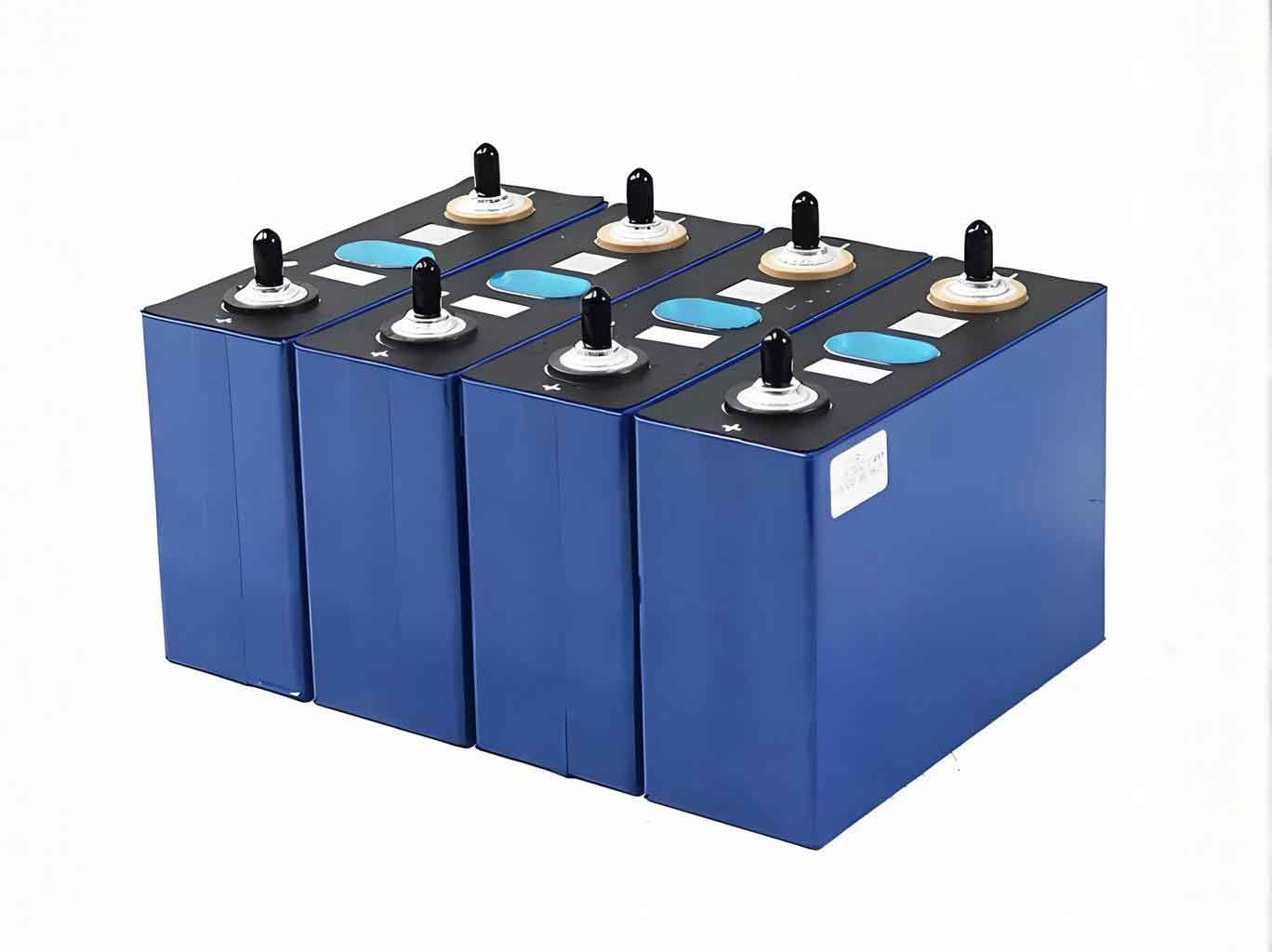
Table 1 summarizes the key parameters of the energy storage cabinet.
| Component | Parameter | Value |
|---|---|---|
| System | Rated energy (kWh) | 200 |
| System | Rated power (0.5C) | 100 kW |
| Battery string | Cell chemistry | LFP |
| Battery string | Nominal cell capacity | 280 Ah |
| Battery string | Number of series cells | 224 |
| Battery string | Nominal total voltage | 716.8 V |
| Battery string | Charge/discharge efficiency | >95% |
| PCS | AC/DC conversion efficiency | >98% |
The passive balancing circuit is shown schematically in Figure 3 of the original work. Each energy storage cell has an independent balancing path; the resistor is placed on the pack sampling control board, and the balancing current is directed away from the cell when the MOSFET is turned on. The AFE chip alternates between voltage measurement and balancing activation in a fixed timing cycle, as illustrated in Figure 5 of the original paper.
SCBS: Self‑Calibration Balance Strategy
Real‑Time Terminal SOC Calibration
The core innovation of SCBS is the online calibration of the SOC–voltage relationship during the final stages of charging and discharging. For LFP energy storage cells, the voltage exhibits a nearly linear change in the SOC ranges of 95%–100% (charging) and 0%–5% (discharging). This linearity allows us to construct a dynamic reference curve using the cell that first reaches the voltage cutoff. During discharge, once the lowest cell voltage drops below 3.1 V, we record the voltage and the accumulated ampere‑hour integral at fixed intervals. The cell that first reaches 2.8 V is designated as the reference cell, and its reference SOC at each moment is calculated as:
$$
\text{SOC}_{ref,dis}(t) = \frac{\text{Th}_{Ah}(t_1) – \text{Th}_{Ah}(t)}{Q_e} \times 100\%
$$
where \(t_1\) is the moment when the system SOC reaches 0% (discharge cutoff), \(\text{Th}_{Ah}(t)\) is the cumulative ampere‑hour integral at time \(t\) (positive for discharge), and \(Q_e\) is the rated system capacity (280 Ah × 224 = 62720 Ah). The ampere‑hour integral is updated as:
$$
\text{Th}_{Ah}(t) = \text{Th}_{Ah}(t_0) + \int_{t_0}^{t} I(\tau) d\tau
$$
Here \(t_0\) is the initial sampling time when the system is first commissioned. Similarly, during charging, when the highest cell voltage exceeds 3.4 V, we monitor the cell that first reaches 3.6 V. The reference SOC for charging is:
$$
\text{SOC}_{ref,cha}(t) = \left(1 – \frac{\text{Th}_{Ah}(t_2) – \text{Th}_{Ah}(t)}{Q_e}\right) \times 100\%
$$
where \(t_2\) is the moment when the system SOC reaches 100% (charge cutoff). By interpolating the voltage of every other energy storage cell against the reference curve \(\mathcal{C}_{ref,dis}\) or \(\mathcal{C}_{ref,cha}\), we obtain the individual SOC at the cutoff moments: \(\text{SOC}_{end,cha}(i)\) and \(\text{SOC}_{end,dis}(i)\). The actual usable capacity of the i‑th energy storage cell is then:
$$
Q_a(i) = \frac{Q_{dis}}{\text{SOC}_{end,cha}(i) – \text{SOC}_{end,dis}(i)}
$$
with \(Q_{dis}\) being the total discharged capacity from full charge to full discharge. The smallest value among \(Q_a(i)\) is denoted \(Q_{cell,min}\). The system can only deliver this amount of energy if all cells are perfectly balanced at the end of charge.
To verify the accuracy of the proposed calibration, we compared it with the conventional offline dynamic terminal voltage–SOC curve method on an energy storage cabinet that had aged by 10% capacity. Table 2 shows the results.
| Condition | Cell Voltage (mV) | True SOC (%) | Offline Curve SOC (%) | Offline Error (%) | Real‑time Calibration SOC (%) | Real‑time Error (%) |
|---|---|---|---|---|---|---|
| Charging | 3445 | 94.7 | 98.7 | 4.0 | 94.4 | 0.3 |
| Charging | 3488 | 96.7 | 99.4 | 2.7 | 96.5 | 0.2 |
| Charging | 3513 | 97.7 | 99.6 | 1.9 | 97.5 | 0.2 |
| Charging | 3542 | 98.7 | 99.8 | 1.1 | 98.5 | 0.2 |
| Charging | 3570 | 99.7 | 99.9 | 0.2 | 99.5 | 0.2 |
| Discharging | 2988 | 7.8 | 2.5 | 5.3 | 7.7 | 0.1 |
| Discharging | 2957 | 5.7 | 1.9 | 3.9 | 5.6 | 0.1 |
| Discharging | 2921 | 3.7 | 1.3 | 2.4 | 3.6 | 0.1 |
| Discharging | 2889 | 2.6 | 0.9 | 1.8 | 2.4 | 0.2 |
| Discharging | 2821 | 0.6 | 0.2 | 0.4 | 0.5 | 0.1 |
The real‑time self‑calibration reduces the maximum SOC error from 5.3% to 0.3%, demonstrating significant improvement, especially for aged energy storage cells.
Full‑Time Adaptive Balancing Control
Once the system meets the conditions that the highest SOC at charge cutoff exceeds 95% and the lowest SOC at discharge cutoff is below 5%, the SCBS algorithm proceeds to identify the cells that need balancing. The goal is to make the SOC of all energy storage cells at the end of charge consistent within 1%. The cell having the minimum SOC at discharge cutoff is used to define the baseline SOC at charge cutoff, denoted as \(\text{SOC}_{base}\). Every energy storage cell whose \(\text{SOC}_{end,cha}(i)\) is larger than \(\text{SOC}_{base}\) is a candidate for balancing. The required balancing duration for the i‑th cell is:
$$
T(i) = \frac{(\text{SOC}_{ref,cha}(t_1) – \text{SOC}_{base}) \times Q_e – \Delta Q}{\theta \times I_b \times 100}
$$
where \(\theta\) is the balancing efficiency, representing the duty cycle of effective balancing within a sampling period (typically 0.8 to 0.9), \(I_b\) is the balancing current (80 mA), and \(\Delta Q\) is a reserve capacity of 1 Ah to prevent over‑balancing. All candidate cells are balanced simultaneously during the entire system operation—whether charging, discharging, or idle—as long as the AFE chip temperature remains below 75 °C. When the temperature exceeds 75 °C, odd‑even interleaved balancing is activated; above 80 °C, balancing is paused until safe temperature returns. After each full charge/discharge cycle, the terminal voltage curves are updated, and the balancing durations are recalculated. This iterative feedback mechanism ensures that the algorithm adapts to aging, resistor degradation, and any calibration errors. Figure 6 in the original paper shows the closed‑loop control flow.
Experimental Setup and Imbalance Construction
Three identical 200 kWh energy storage cabinets (labelled No.1, No.2, No.3) that had been in operation for six months were selected. Their initial parameters are listed in Table 3.
| Cabinet | Initial discharge capacity (Ah) | Max voltage deviation at charge cutoff (mV) |
|---|---|---|
| 1 | 277.9 | 145.7 |
| 2 | 278.5 | 141.2 |
| 3 | 277.4 | 148.2 |
To create a controlled imbalance, we deliberately disabled balancing on cell #11 of every pack, applied continuous full‑time balancing (10 days) to cell #10 of every pack (simulating a weak cell with lower SOC), and applied 5 days of balancing to all other cells. This procedure forced a state where some energy storage cells had significantly lower usable capacity than others. After construction, the voltage distributions at charge and discharge cutoffs are shown in Figure 7 of the original paper. For cabinet No.3, the maximum voltage deviation reached 211.2 mV, and the achievable discharge capacity dropped to 261.5 Ah, representing a 5.3% loss compared to the minimum cell capacity of 275.4 Ah.
Comparative Evaluation of Balancing Strategies
Three balancing strategies were deployed on the three cabinets respectively: cabinet No.1 used MVBS (based on the lowest cell voltage during charging), cabinet No.2 used AVBS (based on the real‑time average voltage of all cells), and cabinet No.3 used SCBS. The strategies ran for 12 days under the same daily 2‑charge‑2‑discharge profile. Table 4 compares the key performance metrics.
| Strategy | Effective balancing hours (h) | Discharge capacity before (Ah) | Discharge capacity after (Ah) | Capacity increase (%) | Max charge‑cutoff voltage deviation before (mV) | Max charge‑cutoff voltage deviation after (mV) | Voltage deviation reduction (mV) |
|---|---|---|---|---|---|---|---|
| MVBS | 5.7 | 262.4 | 262.8 | 0.2 | 192.5 | 191.5 | 1.5 |
| AVBS | 34.9 | 263.1 | 266.2 | 1.2 | 212.4 | 205.1 | 7.3 |
| SCBS | 220 | 261.5 | 277.1 | 5.9 | 211.2 | 150.5 | 60.7 |
The SCBS strategy achieved 220 effective balancing hours—almost 80% of the total time—owing to its full‑time operation. The discharge capacity increased by 5.9%, recovering the cabinet to its initial healthy state. In contrast, MVBS only operated during the short charging periods when voltage differences exceeded 50 mV, resulting in negligible improvement. AVBS improved capacity by only 1.2% because the flat LFP voltage plateau makes it difficult to detect weak cells based on average voltage alone. To further investigate the limitation of AVBS, we extended its runtime on a separate cabinet to 36 days. The results are shown in Table 5.
| Metric | Initial | After 36 days |
|---|---|---|
| Discharge capacity (Ah) | 263.1 | 269.5 |
| Max charge‑cutoff voltage deviation (mV) | 212.4 | 199.0 |
Even after 36 days, AVBS could not drive the system to full minimum‑cell utilization because the average voltage remained too high to trigger balancing for the weakest cells. SCBS, by directly targeting the SOC mismatch, avoids this fundamental limitation.
Energy Loss, Thermal Impact, and Long‑Term Stability
Passive balancing dissipates excess energy from high‑SOC cells as heat. However, in a voltage‑cutoff system, the energy dissipated is exactly the energy that would otherwise be wasted due to premature termination. Therefore, the net energy efficiency of the system is not degraded. The heat generated by the balancing resistors is managed by the BMU board layout; we tested the worst‑case scenario by forcing all 224 cells to balance continuously for 24 hours. The peak AFE chip temperature was 73 °C, well below the 105 °C safety limit. In normal operation, the SCBS algorithm uses temperature feedback to adjust the balancing mode, ensuring thermal safety.
To evaluate long‑term stability, we continued to monitor cabinet No.3 for 120 days after the 12‑day SCBS balancing ended. The discharge capacity and maximum voltage deviation were recorded every 5 days. The data showed that the capacity remained stable at around 277 Ah, and the voltage deviation fluctuated between 148 mV and 155 mV, with no upward trend. This indicates that the SCBS strategy not only restores balance but also maintains it over time.
Scalability and Limitations
The SCBS algorithm does not depend on the specific cell chemistry or module size as long as the terminal voltage exhibits approximately linear behavior in the extreme SOC regions. We tested it on three different series‑connected configurations with 8, 128, and 416 energy storage cells, each with initial imbalance. The results are shown in Table 6.
| Number of cells | Cell capacity (Ah) | Test duration (h) | Max voltage deviation before (mV) | Discharge capacity before (Ah) | Max voltage deviation after (mV) | Discharge capacity after (Ah) |
|---|---|---|---|---|---|---|
| 8 | 314 | 96 | 176.2 | 275.4 | 100.3 | 281.1 |
| 128 | 314 | 120 | 162.3 | 273.5 | 66.8 | 280.6 |
| 416 | 280 | 96 | 117.5 | 272.1 | 50.2 | 277.5 |
In all cases, SCBS effectively reduced voltage deviation and increased the delivered capacity. The improvement is more pronounced for larger modules because the imbalance accumulates over more cells. One limitation is that if the capacity spread among the energy storage cells is large, operating the smallest cell at full utilization every cycle may accelerate its aging. In practice, it is advisable to combine SCBS with a depth‑of‑discharge (DOD) limiter and schedule periodic full‑charge‑discharge calibrations to ensure longevity without sacrificing system economy.
Conclusion
We have presented a novel self‑calibration balancing strategy (SCBS) for series‑connected energy storage systems. By dynamically calibrating the SOC at the end of charge and discharge using the actual terminal voltage curves of the leading cells, and then performing full‑time adaptive equalization, SCBS achieves near‑optimal utilization of the minimum‑capacity cell. Experimental results from three 200 kWh LFP cabinets demonstrate that SCBS increases system discharge capacity by 5.9% in 12 days, which is 4.9 times higher than the improvement obtained with the average‑voltage strategy and far superior to the conventional minimum‑voltage strategy. The algorithm inherently adapts to cell aging, temperature variations, and resistor degradation through iterative feedback. Its energy loss is insignificant because the dissipated energy is otherwise untapped. Thermal safety is ensured by temperature‑aware balancing modes. The strategy scales well to different cell types and system sizes, making it a robust and practical solution for enhancing the capacity and reliability of large‑scale energy storage systems.