
In this paper, we explore the economic viability of a solar photovoltaic ice making system, which integrates renewable energy with refrigeration technology to reduce reliance on conventional power sources. The solar system harnesses solar energy to drive a vacuum ice slurry preparation system, aiming for energy conservation and emission reduction. From a first-person perspective, we develop an economic analysis model, evaluating key metrics such as unit power cost and investment payback period. This analysis provides a foundation for optimizing the entire solar system, ensuring its practical application and scalability. Throughout this discussion, we emphasize the importance of the solar system in achieving sustainable energy goals, and we will frequently reference the solar system to highlight its central role.
The growing demand for clean energy solutions has propelled solar photovoltaic (PV) technology to the forefront of renewable energy applications. Solar systems, particularly those coupled with cooling processes, offer a promising avenue for reducing carbon footprints. Our focus is on a solar system designed for ice making, which combines PV generation with a vacuum-based ice slurry generator. This integration not only leverages abundant solar resources but also addresses the energy-intensive nature of conventional ice production. By analyzing the economics of this solar system, we aim to demonstrate its financial feasibility and identify areas for improvement. The solar system’s performance is critical, and its design directly impacts overall costs and benefits.
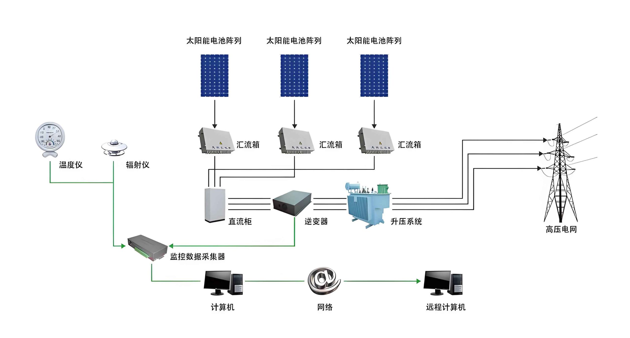
Before delving into the economic model, let us describe the components of the solar photovoltaic ice making system. The system comprises two main subsystems: the solar PV system and the vacuum ice slurry preparation system. The solar PV system includes PV panels, a charge controller, an inverter, and a battery bank. These elements work in tandem to convert sunlight into usable electricity, store excess energy, and ensure stable power supply. The vacuum ice slurry system consists of a vacuum pump, pressure stabilizer, condensation chamber, refrigeration unit, ice slurry generator, ice slurry tank, water tank, pumps, and associated piping. The primary electrical loads are the refrigeration unit, pumps, and vacuum pump, which are powered by the solar system.
To guarantee year-round operation, we adopt a hybrid power supply mode: solar power is prioritized, with grid electricity as a backup. During sunny periods, the PV panels generate direct current (DC), which is partially converted to alternating current (AC) via the inverter for immediate use, while surplus DC is stored in batteries. The controller, inverter, and battery bank collaborate to maintain a stable power output. When solar insufficiency is insufficient, grid power supplements the system, ensuring uninterrupted operation. This design underscores the reliability of the solar system in diverse weather conditions.
The solar system’s efficiency is paramount for economic performance. The PV panels are typically made of polycrystalline silicon, chosen for their balance of cost and efficiency. For instance, in our setup, we use panels with a peak power of 250 W each, arranged in an array to meet the load requirements. The battery bank is sized to support the system for three days without solar input, using maintenance-free batteries with high coulombic efficiency. The inverter and controller incorporate maximum power point tracking (MPPT) to optimize energy harvest from the solar system. Overall, the solar system’s configuration directly influences initial investment and long-term savings.
To assess the economic aspects, we establish a mathematical model based on the solar system’s parameters. The annual electricity generation of the solar system, denoted as \( H_y \) in kilowatt-hours (kWh), is calculated as:
$$ H_y = W D f \eta_b \eta_t = W D \eta $$
where \( W \) is the peak power of the PV panels in kilowatts (kW), \( D \) is the annual peak sun hours, \( f \) is the PV panel performance degradation coefficient (ranging from 0.8 to 0.98), \( \eta_b \) is the battery coulombic efficiency (0.8 to 0.92), \( \eta_t \) is the inverter efficiency (0.9 to 0.96), and \( \eta \) is the overall efficiency converting peak DC power to AC output (0.6 to 0.87). This formula highlights how the solar system’s efficiency factors affect energy yield.
The total initial investment for the solar system, \( BC \) in monetary units, is given by:
$$ BC = W C_0 + (A_1 + A_2 + A_3 + A_4) W C_0 $$
where \( C_0 \) is the price per kilowatt of PV panels, \( A_1 \) is the battery investment coefficient relative to PV panels (0.15 to 0.7), \( A_2 \) is the inverter and controller coefficient (0.15 to 0.5), \( A_3 \) is the mounting structure and cabling coefficient (0.05 to 0.25), and \( A_4 \) accounts for other costs like installation and transportation (0.05 to 0.15). This breakdown shows that the solar system’s cost is dominated by PV panel expenses, which we will analyze later.
The unit power cost, \( C \) in currency per kWh, is a key economic indicator:
$$ C = \frac{C_{tot}}{E_s} $$
where \( C_{tot} \) is the annual total cost, comprising annualized investment cost \( C_{inv} \) and annual operation and maintenance cost \( C_v \), and \( E_s \) is the annual electricity generation. Typically, \( C_v \) is expressed as a coefficient of PV panel cost, ranging from 0.005 to 0.015. This metric helps compare the solar system with conventional grid power.
The investment payback period, \( n \) in years, is calculated as:
$$ n = \frac{BC}{F + a E_s – C_{tot}} $$
where \( F \) represents government subsidies or incentives, and \( a \) is the local grid electricity price. A shorter payback period indicates better economic viability for the solar system.
To illustrate these concepts, we present a detailed calculation based on a case study. The ice making system has a total power demand of 2,850 W, as shown in Table 1. This load determines the sizing of the solar system.
| Equipment | Power (W) |
|---|---|
| Vacuum Pump | 550 |
| Refrigeration Unit | 1,800 |
| Water Pump | 250 |
| Ice Slurry Pump | 250 |
| Total | 2,850 |
The system operates 6 hours per day for 300 days annually, consuming 5,130 kWh of electricity. At a commercial electricity rate of 0.74 currency units per kWh, the annual grid electricity cost would be 3,796.2 currency units. By replacing this with a solar system, we aim to reduce this expense.
Based on the load, we size the PV array. Considering efficiencies \( \eta_b = 0.85 \), \( f = 0.92 \), and \( \eta_t = 0.92 \), the required PV peak power is approximately 3,961 W. We select polycrystalline panels with a peak power of 250 W each, resulting in 16 panels (4 kW total) covering an area of about 25 m². The solar system’s annual generation is estimated using local solar data. For a region with an average solar irradiance of 1,239 W/m² and 6 peak sun hours per day, the annual output is:
$$ H_y = 4 \, \text{kW} \times (6 \, \text{h/day} \times 300 \, \text{days}) \times 0.85 \times 0.92 \times 0.92 \approx 5,176.8 \, \text{kWh} $$
This matches the system’s demand, ensuring self-sufficiency. The battery bank is designed for three days of autonomy, using 24V-200AH batteries. The initial investment breakdown is presented in Table 2, highlighting the cost distribution within the solar system.
| Component | Investment (Currency Units) | Percentage (%) |
|---|---|---|
| PV Panels | 12,160 | 60.4 |
| Inverter and Controller | 2,380 | 11.8 |
| Battery Bank | 3,364 | 16.7 |
| Mounting and Cabling | 1,216 | 6.1 |
| Installation and Other | 1,000 | 5.0 |
| Total | 20,120 | 100 |
Subsidies play a crucial role in enhancing the solar system’s economics. Assuming a national subsidy of 0.42 currency units per kWh and a local subsidy of 0.25 currency units per kWh for distributed PV projects, both applicable for 5 years, the total subsidy over the system’s lifetime is calculated. With annual generation of 5,176.8 kWh, the annual subsidy is:
$$ F_{\text{annual}} = 5,176.8 \times (0.42 + 0.25) = 3,468.5 \, \text{currency units} $$
Over 5 years, this sums to 17,342.5 currency units. The annual total cost \( C_{tot} \) includes annualized investment and O&M. Using a discount rate for annualization, we simplify by assuming straight-line depreciation over 23 years (system lifetime). The annual investment cost is:
$$ C_{inv} = \frac{20,120}{23} \approx 874.8 \, \text{currency units} $$
The annual O&M cost \( C_v \) is taken as 1% of PV panel cost:
$$ C_v = 0.01 \times 12,160 = 121.6 \, \text{currency units} $$
Thus, \( C_{tot} = 874.8 + 121.6 = 996.4 \, \text{currency units} \). The unit power cost is:
$$ C = \frac{996.4}{5,176.8} \approx 0.19 \, \text{currency units per kWh} $$
This is significantly lower than the grid price of 0.74 currency units per kWh, demonstrating the solar system’s cost advantage.
The payback period is computed considering annual savings. Without subsidies, annual savings from grid avoidance are:
$$ \text{Savings} = 5,176.8 \times 0.74 – 996.4 \approx 2,834.0 \, \text{currency units} $$
With subsidies in the first 5 years, the annual net income increases. The payback period \( n \) is:
$$ n = \frac{20,120}{2,834.0 + 3,468.5 – 996.4} \approx 3.2 \, \text{years} $$
This indicates that the solar system recovers its cost in about 3.2 years, which is attractive given its 23-year lifespan.
To deepen the analysis, we explore factors influencing the solar system’s economics. The PV panel investment constitutes 60.4% of the total cost, as shown in Table 2. This highlights that the solar system’s upfront cost is heavily dependent on PV technology prices. Reductions in panel costs, through technological advancements or economies of scale, can drastically improve economic viability. Additionally, the load profile affects panel sizing; for instance, optimizing the ice making process to reduce power demand, such as using more efficient refrigeration units, can lower the required PV capacity and thus initial investment.
The battery bank accounts for 16.7% of the cost. While essential for energy storage, its capacity can be optimized based on local weather patterns and load management strategies. Implementing a hybrid AC/DC operation or integrating smart controllers to minimize battery usage can reduce this expense. Furthermore, the solar system’s performance degradation over time, captured by the coefficient \( f \), impacts long-term generation. Regular maintenance and high-quality components can mitigate this, ensuring sustained output.
Geographical location also plays a role. Solar irradiance varies regionally, affecting the annual peak sun hours \( D \). In areas with higher insolation, the same PV array yields more electricity, improving the unit cost and payback period. For example, if \( D \) increases by 20%, the annual generation rises proportionally, enhancing savings. This underscores the importance of site-specific design for the solar system.
We can formalize some relationships using sensitivity analysis. Let \( \Delta W \) represent a change in PV panel power due to load reduction. The new investment \( BC’ \) is:
$$ BC’ = (W + \Delta W) C_0 + (A_1 + A_2 + A_3 + A_4) (W + \Delta W) C_0 $$
Assuming a linear relationship, the percentage change in investment is approximately proportional to \( \Delta W \). Similarly, variations in subsidy rates \( F \) or electricity prices \( a \) directly affect the payback period. For instance, if subsidies increase by 10%, the payback period shortens, making the solar system more appealing.
To generalize, we can derive an economic optimization model for the solar system. Define the objective function as minimizing the levelized cost of energy (LCOE), which incorporates lifetime costs and generation. LCOE is given by:
$$ \text{LCOE} = \frac{\sum_{t=1}^{T} \frac{C_{inv,t} + C_{v,t}}{(1+r)^t}}{\sum_{t=1}^{T} \frac{E_{s,t}}{(1+r)^t}} $$
where \( T \) is the system lifetime (23 years), \( r \) is the discount rate, \( C_{inv,t} \) and \( C_{v,t} \) are annual investment and O&M costs, and \( E_{s,t} \) is annual electricity generation. For our solar system, assuming constant annual generation and costs, this simplifies to:
$$ \text{LCOE} = \frac{C_{tot}}{E_s} \cdot \frac{1 – (1+r)^{-T}}{r} $$
Using \( r = 5\% \), we get:
$$ \text{LCOE} \approx 0.19 \times \frac{1 – (1.05)^{-23}}{0.05} \approx 0.19 \times 14.856 \approx 2.82 \, \text{currency units per kWh} $$
This is a cumulative measure, but it reaffirms the low energy cost of the solar system compared to grid alternatives.
Another aspect is environmental benefits, which indirectly impact economics through carbon credits or social value. The solar system reduces greenhouse gas emissions by displacing grid electricity, often generated from fossil fuels. Quantifying this, if the grid emission factor is 0.5 kg CO₂ per kWh, the annual emission reduction is:
$$ \text{Reduction} = 5,176.8 \times 0.5 = 2,588.4 \, \text{kg CO₂} $$
Monetizing this at a carbon price of 0.05 currency units per kg CO₂ adds an annual benefit of 129.4 currency units, further improving the solar system’s net income.
We also consider technological trends. PV panel efficiencies are improving, with newer models reaching over 22% conversion rates. Integrating such panels into the solar system can reduce the required area and mounting costs, albeit at a higher per-watt price. A trade-off analysis is essential. For instance, if high-efficiency panels cost 20% more but yield 25% more power, the net effect on investment per kWh might be positive.
Battery technology is evolving rapidly, with lithium-ion batteries offering higher energy density and longer lifespans than traditional lead-acid types. Although initially more expensive, they may reduce long-term replacement costs. Incorporating such advancements into the solar system could enhance reliability and economics.
To provide a comprehensive view, we compare the solar system with conventional ice making systems powered solely by grid electricity. Table 3 summarizes key economic indicators over a 23-year period.
| Indicator | Solar System | Grid-Only System |
|---|---|---|
| Initial Investment (Currency Units) | 20,120 | 0 |
| Annual Electricity Cost (Currency Units) | 996.4 | 3,796.2 |
| Unit Power Cost (Currency Units/kWh) | 0.19 | 0.74 |
| Payback Period (Years) | 3.2 | N/A |
| Lifetime Cost (23 Years, Currency Units) | 22,917.2 | 87,312.6 |
| Net Savings (Currency Units) | 64,395.4 | 0 |
The lifetime cost for the solar system is calculated as \( 20,120 + 23 \times 996.4 = 22,917.2 \), while for the grid-only system, it is \( 23 \times 3,796.2 = 87,312.6 \). The net savings of 64,395.4 currency units clearly favor the solar system, emphasizing its long-term economic superiority.
Moreover, the solar system contributes to energy independence and resilience, especially in remote areas where grid access is unreliable. This added value, though not quantified in monetary terms, enhances its attractiveness. The solar system’s modularity allows for scalability; additional panels can be installed as demand grows, making it a flexible solution.
In terms of implementation, we recommend conducting a detailed feasibility study for each site, considering local solar resources, electricity tariffs, and available incentives. Tools like PVsyst or HOMER can simulate the solar system’s performance and economics under varying conditions. Additionally, engaging with stakeholders to secure financing or partnerships can alleviate upfront costs.
From a policy perspective, governments can further promote such solar systems by increasing subsidies, simplifying permitting processes, and offering tax incentives. These measures would accelerate adoption, driving down costs through market expansion and technological diffusion. The solar system aligns with global sustainability goals, making it a key component in the transition to clean energy.
To conclude, our economic analysis demonstrates that a solar photovoltaic ice making system is financially viable, with a low unit power cost of 0.19 currency units per kWh and a short payback period of 3.2 years. The solar system’s initial investment is largely driven by PV panel costs, but this is offset by substantial savings and subsidies over its lifespan. By optimizing components like batteries and load profiles, the economics can be further improved. We emphasize that the solar system not only offers economic benefits but also environmental advantages, supporting a greener future. As solar technology advances, we anticipate even better performance and cost-effectiveness, making such systems a cornerstone of sustainable refrigeration solutions.
Throughout this discussion, we have consistently highlighted the solar system’s role, underscoring its importance in energy-efficient ice production. Future work could explore integration with other renewables or thermal storage to enhance the solar system’s versatility. We hope this analysis inspires further research and deployment of solar systems in cooling applications, contributing to global energy sustainability.