
The evolution of global power systems is intrinsically linked to the successful integration of renewable energy sources. Among these, the solar system—encompassing both photovoltaic (PV) and concentrating solar power (CSP) technologies—holds unparalleled potential due to the abundance of solar irradiance. However, the inherent intermittency and volatility of PV generation pose significant challenges to grid stability, often forcing conventional thermal units into inefficient and costly deep-cycling operations. This paper delves into the coordinated operation of hybrid PV-CSP systems, presenting a comprehensive optimization model that leverages their complementary characteristics to enhance the overall efficiency, reliability, and economic viability of the solar system integration.
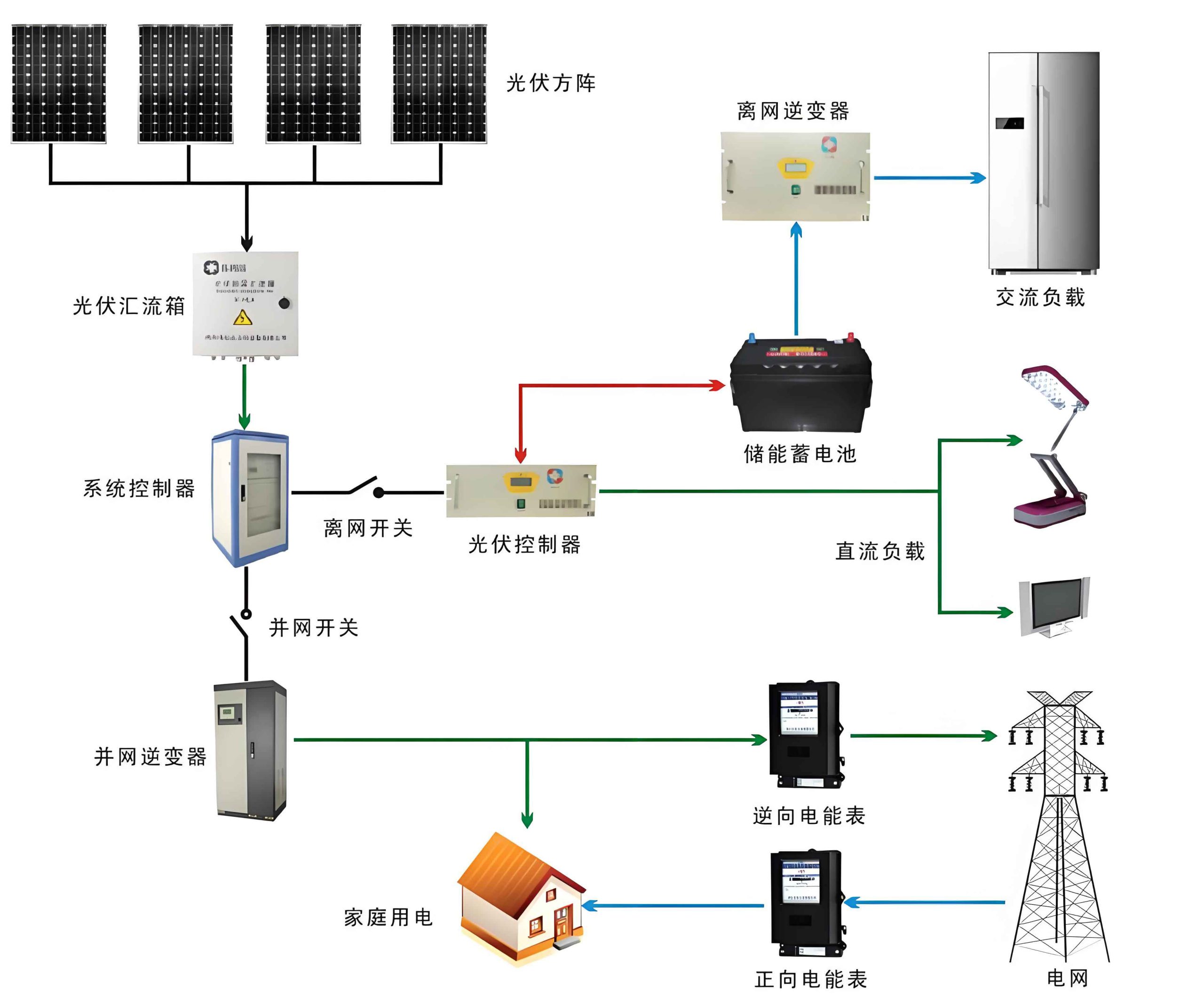
The foundational principle of a coordinated solar system lies in the temporal and operational synergy between its components. PV panels convert sunlight directly into electricity with zero fuel cost but are entirely dependent on real-time solar availability. In contrast, a CSP plant converts solar thermal energy into electricity via a conventional thermodynamic cycle (e.g., a steam turbine). Its defining feature is the integration of a Thermal Energy Storage (TES) system, which decouples energy collection from electricity generation. This storage capability transforms CSP from an intermittent source into a partially dispatchable and flexible asset within the broader solar system. The operational strategy for a hybrid solar system can thus be designed to: 1) utilize PV output as the primary source during peak sunshine hours, 2) use excess solar thermal energy to charge the TES, and 3) dispatch power from the CSP plant’s turbine during evening hours, cloudy periods, or to follow load variations, thereby smoothing the net output profile of the entire solar complex.
Modeling the Hybrid Solar System Components
Photovoltaic Power Generation Model
The output power of a PV system is primarily a function of solar irradiance and ambient temperature. The model for the expected AC power output at time \(t\) can be expressed as:
$$
P^{PV}_{t} = \eta_{inv} \cdot \eta_{other} \cdot P^{STC} \cdot \frac{G_t}{G_{STC}} \cdot [1 + \alpha_{P} (T_{c,t} – T_{STC})]
$$
where:
\(P^{PV}_{t}\): AC power output (kW or MW).
\(\eta_{inv}\): Inverter efficiency.
\(\eta_{other}\): Combined efficiency of other losses (wiring, soiling, etc.).
\(P^{STC}\): Rated power under Standard Test Conditions (STC).
\(G_t\): Solar irradiance on the panel plane at time \(t\) (W/m²).
\(G_{STC}\): Irradiance at STC (1000 W/m²).
\(\alpha_{P}\): Temperature coefficient of power (%/°C).
\(T_{c,t}\): PV cell temperature at time \(t\) (°C).
\(T_{STC}\): Cell temperature at STC (25°C).
The cell temperature \(T_{c,t}\) can be estimated from ambient temperature \(T_{a,t}\) and irradiance:
$$
T_{c,t} = T_{a,t} + \frac{NOCT – 20}{800} \cdot G_t
$$
where \(NOCT\) is the Nominal Operating Cell Temperature. The key constraint for PV is its power limit:
$$
0 \leq P^{PV}_{t} \leq P^{PV}_{max}
$$
Concentrating Solar Power Plant Model
The CSP plant model is more complex due to the multiple energy conversion stages: solar to thermal, thermal storage, and thermal to electrical. A generic model for a CSP plant with TES is presented below.
1. Solar Field Energy Balance: The thermal power collected by the solar field (SF) is:
$$
Q^{SF}_t = \eta_{SF} \cdot A_{SF} \cdot DNI_t – Q^{dump}_t
$$
where \(DNI_t\) is the Direct Normal Irradiance, \(A_{SF}\) is the total mirror aperture area, \(\eta_{SF}\) is the optical efficiency of the solar field, and \(Q^{dump}_t\) is any deliberately dumped or spilled thermal energy.
2. Thermal Storage System (TES) Dynamics: The state of charge (\(SOC^{TES}_t\)) of the TES, typically measured in MWhth, evolves according to:
$$
SOC^{TES}_{t} = SOC^{TES}_{t-1} + \Delta t \cdot \left( \eta_{ch} \cdot Q^{ch}_t – \frac{Q^{disch}_t}{\eta_{disch}} \right) – \Delta t \cdot Q^{loss}_t
$$
where \(Q^{ch}_t\) and \(Q^{disch}_t\) are the charging and discharging thermal powers, \(\eta_{ch}\) and \(\eta_{disch}\) are the respective efficiencies, and \(Q^{loss}_t\) represents standby losses. The SOC is bounded by its capacity:
$$
SOC^{TES}_{min} \leq SOC^{TES}_{t} \leq SOC^{TES}_{max}
$$
3. Power Block (PB) / Turbine: The electrical power output is determined by the thermal power delivered to the power block, \(Q^{PB}_t\):
$$
P^{CSP}_t = \eta_{PB}(Q^{PB}_t) \cdot Q^{PB}_t
$$
where \(\eta_{PB}\) is the thermodynamic efficiency of the power cycle, which itself may be a function of the input thermal power level. The turbine must respect its operational limits:
$$
P^{CSP}_{min} \leq P^{CSP}_t \leq P^{CSP}_{max}
$$
$$
-r^{CSP}_{down} \cdot \Delta t \leq P^{CSP}_t – P^{CSP}_{t-1} \leq r^{CSP}_{up} \cdot \Delta t
$$
where \(r^{CSP}_{up/down}\) are the ramp rate limits.
4. Overall Plant Energy Flow: The thermal power sources and sinks must balance:
$$
Q^{SF}_t = Q^{PB}_t + Q^{ch}_t + Q^{dump}_t
$$
Note that \(Q^{PB}_t\) can be supplied either directly from the solar field, from the TES (\(Q^{disch}_t\)), or from both simultaneously. The dispatch of the hybrid solar system hinges on optimally controlling these flows.
Multi-Objective Optimization for Coordinated Operation
Integrating the hybrid solar system into a grid with conventional generation requires a holistic optimization framework. We formulate a day-ahead scheduling problem with two primary objectives that reflect the value of a well-coordinated solar system.
Objective Functions
Objective 1: Maximize Solar Energy Utilization and Economic Benefit.
This objective aims to maximize the revenue from the solar system while minimizing the total system operating cost.
$$
\max F_1 = \sum_{t=1}^{T} \left( \lambda^{PV}_t P^{PV}_t + \lambda^{CSP}_t P^{CSP}_t \right) – C_{total}
$$
where \(\lambda^{PV}_t\) and \(\lambda^{CSP}_t\) are the economic or environmental benefit coefficients for the solar power, and \(C_{total}\) is the total system cost, which includes:
- Conventional Generation Cost: \(C_{conv} = \sum_{t} \sum_{g} [a_g (P^g_t)^2 + b_g P^g_t + c_g + SU^g_t + SD^g_t]\)
- System Reserve Cost: \(C_{res} = \sum_{t} \sum_{g} (c^{RU} RU^g_t + c^{RD} RD^g_t)\)
- Solar System O&M Cost: \(C_{O&M}^{solar} = \sum_{t} (c^{PV}_{O&M} P^{PV}_t + c^{CSP}_{O&M} P^{CSP}_t)\)
Objective 2: Minimize Net Load Variability.
A key grid service provided by a dispatchable solar system is the reduction of net load ramps. Net load is defined as system load minus the combined output of the PV and CSP plants.
$$
NL_t = L_t – (P^{PV}_t + P^{CSP}_t)
$$
A common metric for variability is the sum of absolute ramps of the net load:
$$
\min F_2 = \sum_{t=1}^{T-1} | NL_{t+1} – NL_t |
$$
Minimizing \(F_2\) leads to a smoother net load profile, reducing the burden on conventional generators for balancing.
Multi-Objective Solution Approach
The two objectives, \(F_1\) (maximize) and \(F_2\) (minimize), are often conflicting. A higher solar yield might increase variability, while excessive smoothing might require curtailing solar energy. A standard approach is the weighted sum method, which scalarizes the problem:
$$
\min \ F = -\omega_1 \cdot \tilde{F_1} + \omega_2 \cdot \tilde{F_2}
$$
where \(\omega_1 + \omega_2 = 1\), and \(\tilde{F_1}\) and \(\tilde{F_2}\) are normalized values of the original objectives (e.g., using min-max normalization) to ensure they are on comparable scales. The weights reflect the system operator’s preference between economic efficiency and grid stability. Alternatively, Pareto front analysis can be conducted to explore the trade-offs.
System-Wide Constraints
The optimization is subject to a full set of physical and operational constraints for the entire power system.
1. Power Balance Constraint:
$$
\sum_{g \in G} P^g_t + P^{PV}_t + P^{CSP}_t = L_t, \quad \forall t
$$
2. Transmission Network Constraints (DC Power Flow Approximation):
$$
P^{flow}_{l,t} = \sum_{n} GSDF_{l,n} \cdot (P^{inj}_{n,t} – L_{n,t}), \quad \forall l, t
$$
$$
-P^{max}_{l} \leq P^{flow}_{l,t} \leq P^{max}_{l}, \quad \forall l, t
$$
where \(GSDF_{l,n}\) is the Generation Shift Distribution Factor for line \(l\) with respect to node \(n\).
3. Conventional Unit Constraints: These include minimum/maximum power limits, ramp rate limits, and minimum up/down time constraints.
4. Hybrid Solar System Constraints: All the PV and CSP model constraints detailed in Section 2 must be satisfied.
Case Study and Performance Analysis
To validate the proposed coordinated optimization model, a case study based on a modified IEEE 30-bus test system is presented. A hybrid solar system comprising a 70 MW PV plant and a 100 MW CSP plant with 6 hours of full-load TES capacity is integrated at specific buses, replacing some conventional capacity. A 24-hour period with typical load and solar resource profiles is analyzed.
| Component | Parameter | Value |
|---|---|---|
| PV Plant | Rated Capacity (\(P^{PV}_{max}\)) | 70 MW |
| O&M Cost (\(c^{PV}_{O&M}\)) | $3/MWh | |
| Benefit Coefficient (\(\lambda^{PV}_t\)) | $21.5/MWh (environmental credit) | |
| CSP Plant | Rated Electrical Capacity (\(P^{CSP}_{max}\)) | 100 MW |
| Minimum Stable Generation (\(P^{CSP}_{min}\)) | 12 MW | |
| Ramp Rate (\(r^{CSP}_{up/down}\)) | 12 MW/5-min | |
| TES Capacity (\(SOC^{TES}_{max}\)) | 1000 MWhth | |
| O&M Cost (\(c^{CSP}_{O&M}\)) | $2/MWh | |
| Benefit Coefficient (\(\lambda^{CSP}_t\)) | $21.5/MWh |
The optimization was solved for different weight combinations (\(\omega_1, \omega_2\)). Key results from a balanced scenario (\(\omega_1=0.5, \omega_2=0.5\)) are summarized below.
| Metric | Scenario A: Reference (No Solar) | Scenario B: PV Only (70 MW) | Scenario C: Coordinated PV-CSP (170 MW) |
|---|---|---|---|
| Total Solar Energy Utilized (MWh) | 0 | 813 | 1,618 |
| Total System Cost ($) | 1,245,000 | 1,181,000 | 1,148,000 |
| Net Load Ramp Index (MW) | 1,850 | 2,120 (Increased volatility) | 1,560 |
| Conventional Unit Starts/Stops | 12 | 18 | 8 |
| Peak Ramp Demand on Thermal Units (MW/h) | 95 | 135 | 72 |
The results clearly demonstrate the advantages of the coordinated solar system (Scenario C):
- Enhanced Solar Utilization: The CSP’s TES allows the capture and time-shift of solar energy, nearly doubling the utilized solar MWh compared to the PV-only scenario. This significantly reduces “solar curtailment.”
- Improved Grid Stability: The coordinated system achieves the lowest Net Load Ramp Index. The CSP plant effectively smoothens the combined output: it charges storage and slightly reduces output during midday PV peaks, and discharges to generate power in the evening, creating a much flatter net load profile.
- Economic and Operational Benefits: Despite higher capital cost, the operational flexibility leads to the lowest total system cost. The reduced net load volatility decreases the number of stressful starts/stops and high ramping events for conventional units, lowering wear-and-tear and fuel costs associated with inefficient operating points.
The dispatch profile visually confirms this synergy. During hours 10-15, PV output is high. The CSP plant operates at a moderate level, using part of the solar thermal energy for immediate generation and storing the rest. After sunset (hour 18 onwards), PV output falls to zero, but the CSP plant dispatches power at near its rated capacity from the stored energy, effectively providing firm, renewable capacity to meet the evening load peak.
Future Perspectives and Conclusion
The coordinated operation of photovoltaic and concentrating solar power plants represents a paradigm shift in how we design and manage solar-dominant power systems. By moving beyond viewing PV and CSP in isolation, their integration into a single, strategically operated hybrid solar system unlocks capabilities that address the core challenges of renewable integration: variability, uncertainty, and lack of dispatchability.
The optimization model presented demonstrates that the value of such a solar system extends far beyond the sum of its parts. Key findings include:
- The dispatchability afforded by CSP’s thermal storage is a critical complement to variable PV generation, enabling true firm capacity from solar resources.
- Multi-objective optimization allows system operators to balance economic drivers (maximizing solar revenue, minimizing system cost) with technical performance goals (minimizing net load volatility, reducing thermal unit stress).
- This coordination leads to tangible benefits: increased total solar energy harvest, reduced system operating costs, and enhanced grid stability through a smoother net load profile.
Future research directions for advanced solar systems should focus on:
- Advanced Forecasting and Stochastic Optimization: Incorporating probabilistic forecasts of DNI and PV irradiance into the scheduling model to better manage uncertainty.
- Hybridization with Other Storage: Co-optimizing CSP’s inherent thermal storage with co-located battery energy storage systems (BESS) for sub-hourly frequency regulation and black-start capabilities.
- Market Participation Strategies: Developing bidding strategies for hybrid solar systems in electricity markets, capturing value from energy, capacity, and ancillary service products.
- Distributed and Community-Scale Integration: Exploring the potential of smaller-scale, distributed CSP-PV hybrids for microgrids and industrial applications.
In conclusion, the synergistic integration of PV and CSP into a unified, optimally dispatched solar system is not merely a technical option but a strategic imperative for achieving high-penetration renewable targets. It paves the way for a more reliable, resilient, and cost-effective clean energy grid, solidifying the role of solar power as a cornerstone of the global energy transition.