
In recent years, the rapid development of renewable energy has led to significant challenges in grid integration, particularly with the curtailment of solar and wind power. As a researcher focused on energy storage solutions, we have been exploring hydrogen energy storage as a promising approach to address this issue. Among various technologies, direct coupling of photovoltaic (PV) arrays with proton exchange membrane (PEM) water electrolyzers offers a simplified and efficient method for solar hydrogen production. This article presents our comprehensive analysis and optimization strategies for such solar systems, aiming to minimize energy losses and maximize solar utilization. We will delve into mathematical modeling, operational impacts, and tuning methods, all while emphasizing the importance of well-designed solar systems in the renewable energy landscape.
The core idea behind direct coupling solar systems is to connect PV panels directly to PEM electrolyzers without intermediate power conversion devices like DC-DC converters or maximum power point tracking (MPPT) controllers. This not only reduces system cost and complexity but also avoids additional energy losses associated with power electronics. However, the intermittent nature of solar irradiance and temperature variations can cause mismatches between the PV output and the electrolyzer load, leading to suboptimal operation. Our work focuses on optimizing these solar systems through structural adjustments and operational tuning, ensuring that the system operates near the maximum power point (MPP) of the PV array under varying conditions.
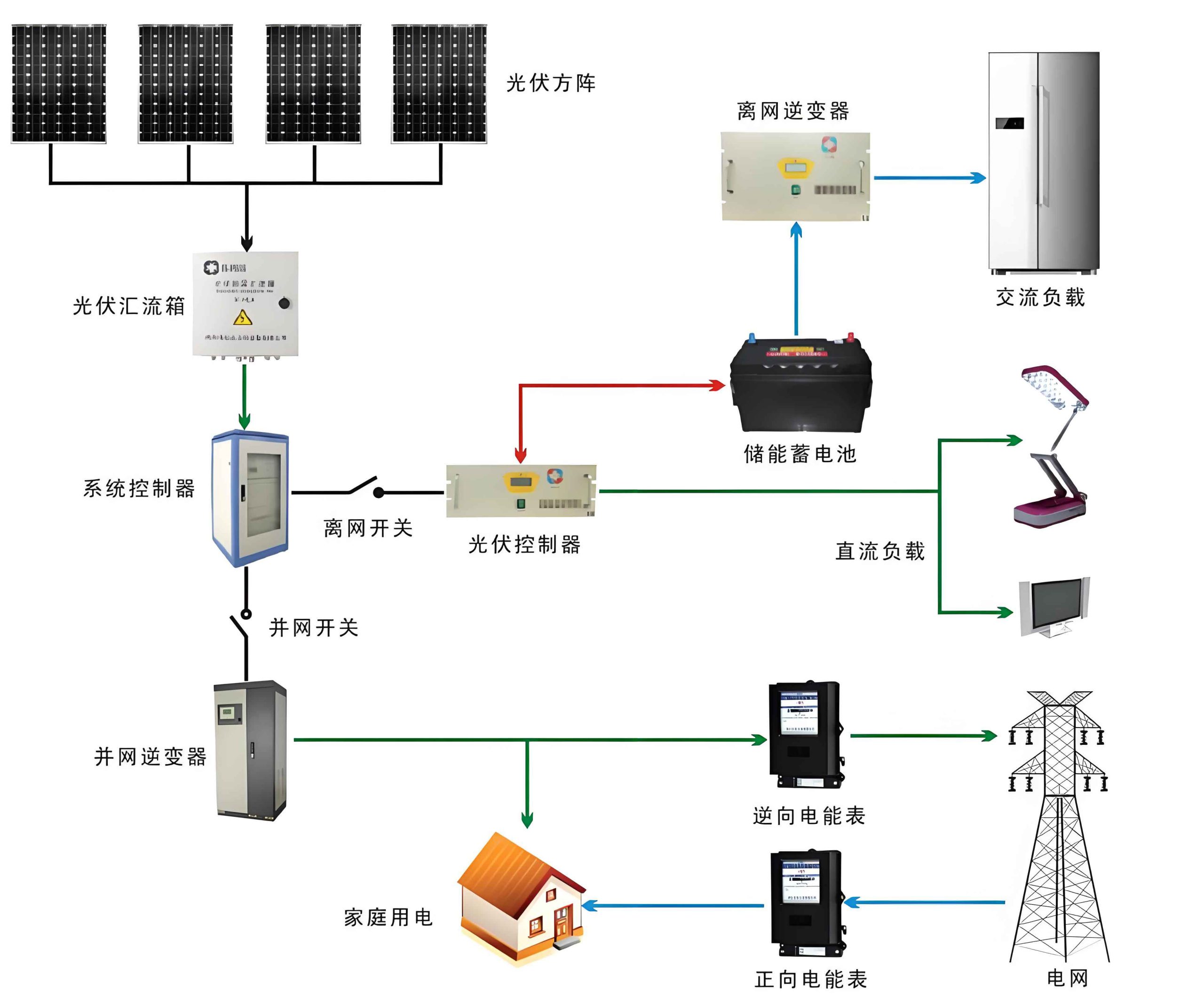
To analyze the performance of direct coupling solar systems, we developed detailed mathematical models for the PV array and the PEM electrolyzer. The PV model is based on a double-diode equivalent circuit, which accurately represents the current-voltage characteristics under different solar irradiance and temperature conditions. The output current \( I \) of a solar cell can be expressed as:
$$ I = I_{\text{ph}} – I_{01} \left[ \exp\left( \frac{V + I R_s}{n_1 k T / q} \right) – 1 \right] – I_{02} \left[ \exp\left( \frac{V + I R_s}{n_2 k T / q} \right) – 1 \right] – \frac{V + I R_s}{R_p} $$
where \( I_{\text{ph}} \) is the photocurrent, \( I_{01} \) and \( I_{02} \) are reverse saturation currents, \( R_s \) and \( R_p \) are series and shunt resistances, \( n_1 \) and \( n_2 \) are ideality factors, \( k \) is Boltzmann’s constant, \( T \) is the cell temperature, and \( q \) is the electron charge. For a PV array consisting of \( N_s \) series and \( N_p \) parallel modules, the total voltage and current are scaled accordingly:
$$ V_{\text{array}} = N_s V, \quad I_{\text{array}} = N_p I $$
The photocurrent and open-circuit voltage vary with solar irradiance \( S \) and temperature \( T_{\text{PV}} \):
$$ I_{\text{sc}} = I_{\text{sc,STC}} \left[ 1 + \alpha_{\text{sc}} (T_{\text{PV}} – T_{\text{PV,STC}}) \right] \frac{S}{S_{\text{STC}}} $$
$$ V_{\text{oc}} = V_{\text{oc,STC}} \left[ 1 + \beta_{\text{oc}} (T_{\text{PV}} – T_{\text{PV,STC}}) \right] + \gamma \ln\left( \frac{S}{S_{\text{STC}}} \right) $$
Here, STC denotes standard test conditions (1000 W/m², 25°C), and \( \alpha_{\text{sc}} \), \( \beta_{\text{oc}} \), and \( \gamma \) are empirical coefficients. These equations allow us to simulate the PV output for any weather condition, which is crucial for designing robust solar systems.
For the PEM electrolyzer, the operating voltage \( V_{\text{WE}} \) is composed of the reversible voltage and overpotentials:
$$ V_{\text{WE}} = V_0 + V_{\text{act}} + V_{\text{ohm}} + V_{\text{diff}} $$
where \( V_0 \) is the open-circuit voltage given by the Nernst equation, \( V_{\text{act}} \) is the activation overpotential, \( V_{\text{ohm}} \) is the ohmic overpotential, and \( V_{\text{diff}} \) is the diffusion overpotential (often negligible). The reversible voltage depends on temperature \( T_{\text{WE}} \) and pressures:
$$ V_0 = 1.229 – 0.9 \times 10^{-3} (T_{\text{WE}} – 298) + \frac{R T_{\text{WE}}}{2F} \ln\left( \frac{P_{\text{H}_2} P_{\text{O}_2}^{0.5}}{P_{\text{H}_2\text{O}}} \right) $$
with \( R \) as the gas constant, \( F \) as Faraday’s constant, and \( P_{\text{H}_2} \), \( P_{\text{O}_2} \), \( P_{\text{H}_2\text{O}} \) as partial pressures of hydrogen, oxygen, and water, respectively. The ohmic overpotential is calculated from the membrane resistance:
$$ V_{\text{ohm}} = i \frac{\delta}{\sigma} $$
where \( i \) is the current density, \( \delta \) is membrane thickness, and \( \sigma \) is ionic conductivity. The activation overpotential for anode and cathode are modeled using Butler-Volmer expressions:
$$ V_{\text{act,an}} = \frac{R T_{\text{WE}}}{F} \sinh^{-1}\left( \frac{i}{2 i_{\text{an0}}} \right), \quad V_{\text{act,ca}} = \frac{R T_{\text{WE}}}{F} \sinh^{-1}\left( \frac{i}{2 i_{\text{ca0}}} \right) $$
The exchange current densities \( i_{\text{an0}} \) and \( i_{\text{ca0}} \) vary with temperature and catalyst properties. These models enable us to predict the electrolyzer’s I-V curve, which is essential for coupling with the PV array in solar systems.
The efficiency of the direct coupling solar system is evaluated through several metrics. The PV conversion efficiency \( \eta_{\text{PV}} \) is the ratio of maximum PV power to incident solar energy:
$$ \eta_{\text{PV}} = \frac{P_{\text{m}}}{S A_{\text{PV}} N_s N_p} $$
where \( P_{\text{m}} \) is the maximum power, and \( A_{\text{PV}} \) is the area per module. The coupling efficiency \( \eta_{\text{C}} \) measures how close the operating point is to the MPP:
$$ \eta_{\text{C}} = \frac{P_{\text{c}}}{P_{\text{m}}} $$
with \( P_{\text{c}} \) as the actual power delivered to the electrolyzer. The electrolyzer efficiency \( \eta_{\text{WE}} \) relates the hydrogen production rate to input power:
$$ \eta_{\text{WE}} = \frac{\dot{n}_{\text{H}_2} \text{LHV}_{\text{H}_2}}{P_{\text{c}}} $$
where \( \dot{n}_{\text{H}_2} = \frac{N_{\text{cell}} I}{2F} \) is the hydrogen molar flow rate, \( \text{LHV}_{\text{H}_2} \) is the lower heating value, and \( N_{\text{cell}} \) is the number of electrolyzer cells. Finally, the overall system efficiency \( \eta_{\text{sys}} \) combines these factors:
$$ \eta_{\text{sys}} = \eta_{\text{PV}} \eta_{\text{C}} \eta_{\text{WE}} = \frac{\dot{n}_{\text{H}_2} \text{LHV}_{\text{H}_2}}{S A_{\text{PV}} N_s N_p} $$
These equations provide a framework for assessing and optimizing solar systems. To illustrate typical parameters, we summarize key values used in our simulations in the following table.
| Component | Parameter | Value |
|---|---|---|
| PV Module | Open-circuit voltage, \( V_{\text{oc,STC}} \) | 0.58 V |
| Short-circuit current, \( I_{\text{sc,STC}} \) | 6.2 A | |
| MPP voltage, \( V_{\text{mp,STC}} \) | 0.5 V | |
| MPP current, \( I_{\text{mp,STC}} \) | 5.6 A | |
| Area per module, \( A_{\text{PV}} \) | 0.015625 m² | |
| PEM Electrolyzer | Active area, \( A \) | 24 cm² |
| Membrane thickness, \( \delta \) | 200 μm | |
| Operating temperature range, \( T_{\text{WE}} \) | 10–90°C | |
| Operating pressure range, \( P_{\text{ca}} \) | 1–70 atm |
Our analysis reveals that weather conditions significantly impact the performance of direct coupling solar systems. Solar irradiance and ambient temperature affect the PV output, causing the operating point to deviate from the MPP. For instance, as irradiance decreases from 1000 W/m² to 200 W/m², the power mismatch increases from 0.6% to 14.2%, reducing coupling efficiency. Temperature variations also play a role; a rise from 20°C to 40°C can lead to a power deviation of up to 3.6%. These mismatches underscore the need for adaptive strategies in solar systems to maintain high efficiency under fluctuating environmental conditions.
To mitigate these issues, we propose two optimization approaches: structural tuning and operational tuning. Structural tuning involves adjusting the series-parallel configuration of the PV array and the number of electrolyzer cells. This serves as a “coarse adjustment” to align the I-V curves of the PV and electrolyzer. For example, with a fixed total of 60 PV cells, different combinations of \( N_s \) and \( N_p \) yield varying coupling efficiencies. The following table summarizes the effects of structural changes on system performance under standard conditions.
| \( N_s \) | \( N_p \) | \( N_{\text{cell}} \) | \( \eta_{\text{PV}} \) (%) | \( \eta_{\text{C}} \) (%) | \( \eta_{\text{WE}} \) (%) | \( \eta_{\text{sys}} \) (%) |
|---|---|---|---|---|---|---|
| 60 | 1 | 16 | 17.9 | 99.6 | 65.6 | 11.7 |
| 30 | 2 | 7 | 17.9 | 97.8 | 61.9 | 10.9 |
| 20 | 3 | 5 | 17.9 | 97.4 | 60.0 | 10.5 |
| 15 | 4 | 3 | 17.9 | 92.8 | 56.8 | 9.4 |
| 12 | 5 | 3 | 17.9 | 84.6 | 57.5 | 8.7 |
As shown, increasing the series count \( N_s \) generally improves coupling efficiency, but it also reduces operating current, which may affect the economic viability of the solar system due to lower current densities in the electrolyzer. Therefore, structural tuning must balance efficiency with practical constraints.
Operational tuning, on the other hand, involves adjusting the electrolyzer operating temperature \( T_{\text{WE}} \) to fine-tune the system. Since the electrolyzer voltage decreases with temperature, raising \( T_{\text{WE}} \) can shift the operating point toward the MPP when irradiance drops. This “fine adjustment” can achieve near-perfect coupling efficiency under varying irradiance levels. For example, with \( N_s = 30 \), \( N_p = 1 \), and \( N_{\text{cell}} = 8 \), we can maintain \( \eta_{\text{C}} = 100\% \) across different irradiance values by modulating \( T_{\text{WE}} \), as demonstrated below.
| \( S \) (W/m²) | \( T_{\text{WE}} \) (°C) | \( \eta_{\text{PV}} \) (%) | \( \eta_{\text{C}} \) (%) | \( \eta_{\text{WE}} \) (%) | \( \eta_{\text{sys}} \) (%) |
|---|---|---|---|---|---|
| 1000 | 39.9 | 17.9 | 100 | 66.8 | 12.0 |
| 800 | 54.8 | 17.2 | 100 | 69.6 | 12.0 |
| 600 | 70.0 | 16.4 | 100 | 72.8 | 12.0 |
| 400 | 83.2 | 15.7 | 100 | 76.5 | 12.0 |
| 200 | 91.0 | 14.8 | 100 | 80.8 | 12.0 |
Interestingly, the overall system efficiency \( \eta_{\text{sys}} \) remains constant at 12.0% in this ideal case because the ratio of operating current to irradiance is fixed at the MPP. However, temperature tuning has limits; if the structural mismatch is severe (e.g., too few electrolyzer cells), adjusting temperature within practical ranges may not suffice to reach the MPP. Thus, a combined approach is essential for robust solar systems.
We further explored the influence of electrolyzer pressure on system performance. Higher cathode pressures, while beneficial for hydrogen storage, increase the electrolyzer voltage due to the Nernst effect, potentially exacerbating coupling mismatches. For instance, at 80°C and 1 atm anode pressure, raising the cathode pressure from 1 atm to 70 atm increases the voltage by approximately 0.2 V at typical current densities. This must be accounted for in the design of solar systems intended for high-pressure hydrogen output.
In practice, implementing these optimizations requires real-time monitoring and control. For solar systems deployed in remote areas, simplicity and reliability are key. Direct coupling eliminates complex electronics, but adaptive tuning mechanisms—such as switching electrolyzer cells or modulating temperature via thermal management—can enhance performance. We envision smart solar systems that autonomously adjust configuration and operation based on weather forecasts and sensor data, maximizing hydrogen yield while minimizing losses.
Our conclusions emphasize the importance of holistic design for direct coupling solar systems. First, weather-induced variations in irradiance and temperature can cause significant mismatches, reducing solar utilization. Second, structural tuning through PV array configuration and electrolyzer cell count provides a coarse alignment to bring the operating point near the MPP. Third, operational tuning via electrolyzer temperature adjustment offers fine control to achieve optimal coupling. Together, these strategies minimize energy losses and ensure efficient hydrogen production. Future work will focus on experimental validation and economic analysis to advance the deployment of such solar systems in renewable energy networks.
Throughout this discussion, we have highlighted the critical role of solar systems in enabling sustainable hydrogen production. By integrating photovoltaic generation with electrolysis, these systems contribute to energy storage and grid stability. The optimization methods presented here are applicable to a wide range of solar systems, from small-scale off-grid installations to large solar farms. As renewable energy penetration grows, advancing direct coupling technology will be vital for harnessing solar power effectively and reducing curtailment. We believe that continued research and innovation in solar systems will pave the way for a cleaner energy future.