
The pursuit of efficient and reliable renewable energy solutions has placed photovoltaic (PV) technology at the forefront of modern power engineering. When constructing a photovoltaic solar system, a significant challenge arises from the highly variable output power of PV cells, which depends substantially on incident irradiance and operating temperature. Utilizing a real, physical PV array for research and development, especially for systems rated at hundreds of watts or higher, involves prohibitive costs. To reduce investment, enhance feasibility, and accelerate the design process, the development of an accurate and computationally efficient PV array simulation model becomes paramount. A robust model can simulate the characteristics, load capability, and overall performance of a PV array under diverse conditions of sunlight, temperature, and electrical configuration. This capability drastically shortens the research cycle for any photovoltaic solar system, improves research efficiency, and increases the credibility of findings. Therefore, establishing a reliable PV array model is not merely beneficial but essential for practical engineering work. This article, from my perspective as a practitioner in the field, details a method for simulating a practical PV array model within the PSCAD/EMTDC electromagnetic transient simulation environment, a tool critical for analyzing the dynamic behavior of integrated power systems.
The core of any photovoltaic solar system is the PV cell, a semiconductor device that converts sunlight directly into electricity via the photovoltaic effect. The fundamental electrical behavior of a PV cell is best understood through its equivalent circuit, which includes a photocurrent source, a diode representing the PN junction, and series and shunt resistances. To derive a practical mathematical expression for simulation, certain simplifications are applied to this detailed model. A widely adopted and effective simplified I-V characteristic equation is given by:
$$I = I_{sc} \times \left[1 – B_1 \times \left(e^{V/(B_2 V_{oc})} – 1\right)\right]$$
where \(I\) is the output current of the PV cell, \(I_{sc}\) is the short-circuit current, \(V\) is the output voltage, \(V_{oc}\) is the open-circuit voltage, and \(B_1\), \(B_2\) are empirical coefficients to be determined.
The coefficients \(B_1\) and \(B_2\) are solved using the key operational parameters at the Maximum Power Point (MPP). At the MPP, we have \(I = I_m\) and \(V = V_m\), where \(I_m\) is the MPP current and \(V_m\) is the MPP voltage. An approximation holds at this point:
$$e^{V_m / (B_2 V_{oc})} \gg 1 \quad \text{so} \quad e^{V_m / (B_2 V_{oc})} – 1 \approx e^{V_m / (B_2 V_{oc})}$$
Using this approximation within the I-V equation allows us to solve for the coefficients:
$$B_1 = \left(1 – \frac{I_m}{I_{sc}}\right) \times e^{-V_m / (B_2 V_{oc})}$$
$$B_2 = \left(\frac{V_m}{V_{oc}} – 1\right) \times \left[\ln\left(1 – \frac{I_m}{I_{sc}}\right)\right]^{-1}$$
Therefore, once the four key parameters \((I_{sc}, I_m, V_{oc}, V_m)\) are specified for a reference condition, \(B_1\) and \(B_2\) become constants, fully defining the I-V curve for that condition via the primary equation. This forms the foundational model for a single cell, which is then scaled to represent modules and arrays within a complete photovoltaic solar system.
A critical aspect of modeling a real-world photovoltaic solar system is accounting for environmental variability. The cell’s parameters are not static; they change with irradiance (\(S\)) and cell temperature (\(T\)). Given new operating conditions (\(S, T\)), the updated parameters \((I_{sc-new}, I_{m-new}, V_{oc-new}, V_{m-new})\) can be calculated from the reference parameters \((I_{sc}, I_m, V_{oc}, V_m\) at \(S_{ref}, T_{ref})\). The defining equations are:
$$\Delta T = T – T_{ref}$$
$$\Delta S = \frac{S}{S_{ref}} – 1$$
$$I_{sc-new} = I_{sc} \times \frac{S}{S_{ref}} \times (1 + a \Delta T)$$
$$I_{m-new} = I_m \times \frac{S}{S_{ref}} \times (1 + a \Delta T)$$
$$V_{oc-new} = V_{oc} \times \left[(1 – c \Delta T) \times \ln(e + b \Delta S)\right]$$
$$V_{m-new} = V_m \times \left[(1 – c \Delta T) \times \ln(e + b \Delta S)\right]$$
Here, \(a\), \(b\), and \(c\) are intrinsic coefficients specific to the PV cell technology, governing its temperature and irradiance sensitivity. With these new parameters, new coefficients \(B_{1-new}\) and \(B_{2-new}\) are computed, allowing the model to generate accurate I-V curves for any given environmental input. This dynamic adjustment is what makes the model invaluable for simulating the non-linear, time-varying output of a photovoltaic solar system.
| Symbol | Description | Unit |
|---|---|---|
| \(I, V\) | Cell output current and voltage | A, V |
| \(I_{sc}, V_{oc}\) | Short-circuit current and open-circuit voltage | A, V |
| \(I_m, V_m\) | Current and voltage at maximum power point (MPP) | A, V |
| \(P_m\) | Maximum power (\(I_m \times V_m\)) | W |
| \(S, T\) | Irradiance and cell temperature | W/m², °C |
| \(S_{ref}, T_{ref}\) | Reference irradiance and temperature | W/m², °C |
| \(B_1, B_2\) | Empirical coefficients for I-V curve shape | Dimensionless |
| \(a, b, c\) | Temperature and irradiance coefficients | 1/°C, Dimensionless, 1/°C |
The output characteristics of a PV module, which is a series-parallel combination of cells, exhibit a distinct single-peak (convex) shape for both I-V and P-V curves. At a constant temperature, increasing irradiance raises both the short-circuit current and the maximum power proportionally, while the open-circuit voltage increases only logarithmically. Conversely, at constant irradiance, increasing temperature significantly reduces the open-circuit voltage and slightly increases the short-circuit current, leading to a notable decrease in maximum power. This non-linear, condition-dependent behavior underscores the necessity of Maximum Power Point Tracking (MPPT) in any efficient photovoltaic solar system to ensure optimal energy harvest.
The principle of MPPT is based on the unique P-V curve. For a given condition, there exists one specific operating voltage \(V_m\) that yields the maximum possible output power \(P_m\). If the operating voltage is less than \(V_m\), power increases with increasing voltage. If the voltage is greater than \(V_m\), power decreases with increasing voltage. Therefore, by actively controlling the operating point (typically by adjusting the duty cycle of a downstream DC-DC converter), the system can be forced to operate at or very near this optimal point. Numerous algorithms exist, with the Perturb and Observe (P&O) method being one of the most common due to its simplicity.
In my implementation, I employ an improved P&O algorithm with an adaptive step-change mechanism based on a voltage threshold. The basic P&O algorithm works by periodically perturbing (slightly increasing or decreasing) the operating voltage and observing the resulting change in output power. If the power increases, the perturbation continues in the same direction; if it decreases, the direction of perturbation is reversed. However, the classic method suffers from a trade-off: a large perturbation step size leads to fast tracking under rapidly changing conditions but causes significant steady-state oscillation around the MPP, wasting energy. A small step size minimizes steady-state loss but is too slow to track rapid irradiance changes, such as those caused by moving clouds.
The improved algorithm introduces a voltage-based judgment. It continuously compares the present operating voltage \(V\) with the estimated MPP voltage \(V_m\). A threshold value \(th\) is defined. The algorithm’s logic is summarized below:
| Step | Action | Logic |
|---|---|---|
| 1 | Measure | Sample present voltage \(V_k\) and current \(I_k\). Calculate power \(P_k = V_k \times I_k\). |
| 2 | Compare | Compare \(P_k\) with previous power \(P_{k-1}\). |
| 3 | Determine Step Size | Calculate \(|V_k – V_m|\). If \(|V_k – V_m| \leq th\), use a small perturbation step \(\Delta V_{small}\). Otherwise, use a large step \(\Delta V_{large}\). |
| 4 | Perturb | If \(P_k > P_{k-1}\), keep the previous perturbation direction. If \(P_k < P_{k-1}\), reverse the perturbation direction. Apply the chosen step size \(\Delta V\) to adjust the voltage reference \(V_{ref}\). |
| 5 | Update & Iterate | Store \(V_k\) and \(P_k\) as \(V_{k-1}\) and \(P_{k-1}\) for the next cycle. Update the internal estimate of \(V_m\) based on the tracked operating point. Repeat from Step 1. |
This method effectively decouples the tracking speed from the steady-state accuracy. Far from the MPP, it takes large, swift steps to converge quickly. As it approaches the vicinity of the MPP (defined by the threshold \(th\)), it switches to fine, small steps to minimize oscillation and power loss. This adaptive behavior is crucial for maximizing the long-term yield of a grid-connected photovoltaic solar system.
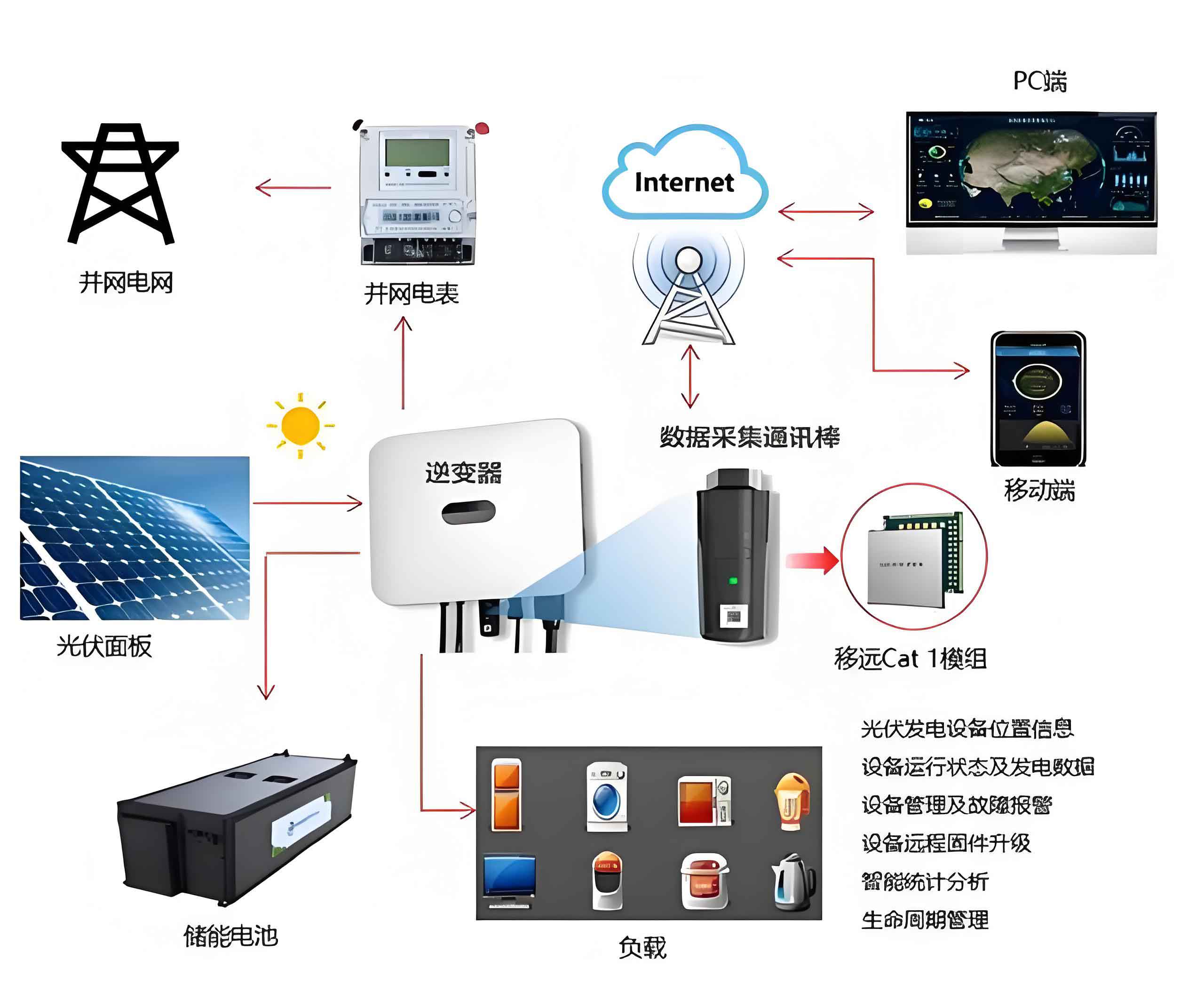
To integrate the generated DC power into the AC grid, a power electronic interface is required. The typical architecture for a three-phase grid-connected photovoltaic solar system (GCPS) consists of the PV array, a DC-link capacitor, a voltage-source converter (VSC) inverter, an LCL or LC filter, and the utility grid. The inverter performs the dual functions of DC-AC conversion and sophisticated grid interaction control. Since both the inverter output and the grid are voltage sources, they cannot be directly connected. The connecting inductors (part of the filter) are essential to control the power flow.
The real and reactive power (\(P\) and \(Q\)) injected into the grid can be controlled by manipulating the amplitude and phase of the inverter’s output voltage relative to the grid voltage. For a simplified system with an inductive link \(X_L\), the power equations are:
$$P = \frac{U_g \times U_s \times \sin \delta}{X_L}$$
$$Q = \frac{U_g \times (U_s \cos \delta – U_g)}{X_L}$$
where \(U_g\) is the grid voltage, \(U_s\) is the fundamental output voltage of the inverter, and \(\delta\) is the power angle (phase difference). For small angles (\(\delta < 5^\circ\)), these simplify to:
$$P \approx \frac{U_g \times U_s \times \delta}{X_L}$$
$$Q \approx \frac{U_g \times (U_s – U_g)}{X_L}$$
This shows that active power flow \(P\) is primarily controlled by the phase angle \(\delta\), while reactive power flow \(Q\) is controlled by the voltage amplitude difference. To implement this control digitally, a synchronous rotating d-q reference frame transformation is employed. This transformation locks onto the grid voltage frequency, converting the three-phase AC quantities into DC quantities in the d-q domain, which vastly simplifies the design of Proportional-Integral (PI) controllers.
The overall inverter control structure typically features an outer power control loop and an inner current control loop. The outer loop takes the MPPT-derived active power reference \(P_{ref}\) and a desired reactive power reference \(Q_{ref}\) (often set to zero for unity power factor) and generates the corresponding d-axis and q-axis current references (\(i_{d\_ref}, i_{q\_ref}\)). The inner fast-current control loop then forces the actual measured d-q currents to follow these references. The output of the current controllers provides the d-q voltage references (\(v_d^*, v_q^*\)) for the inverter’s Pulse Width Modulation (PWM) scheme, such as Space Vector PWM (SVPWM). The current control equations in the d-q frame, after decoupling the cross-coupling terms, are:
$$v_d^* = v_{sd} – \omega L i_q + \left(K_{p} + \frac{K_{i}}{s}\right)(i_{d\_ref} – i_d)$$
$$v_q^* = v_{sq} + \omega L i_d + \left(K_{p} + \frac{K_{i}}{s}\right)(i_{q\_ref} – i_q)$$
Here, \(v_{sd}\) and \(v_{sq}\) are the grid voltage d-q components, \(\omega\) is the grid angular frequency, \(L\) is the filter inductance, and \(K_p\), \(K_i\) are the PI controller gains. This cascaded control structure ensures precise and independent control of active and reactive power, which is a fundamental requirement for the stable and compliant operation of a modern photovoltaic solar system.
To validate the complete model—encompassing the PV array, the improved MPPT algorithm, and the grid-tied inverter control—a dynamic simulation study was conducted in PSCAD/EMTDC. The MPPT algorithm was implemented as a custom component using C-language for the logical operations, storing previous voltage and power values to make decisions for the next time step. The simulation scenario involved a step change in solar irradiance to test the system’s dynamic response. Initially, the irradiance was set at 300 W/m². At time t = 4 seconds, it was stepped up to 1000 W/m². Subsequently, at t = 7 seconds, it was stepped down to 500 W/m².
The simulation results clearly demonstrate the effectiveness of the modeling and control approach. The PV array’s output power, dictated by its inherent diode characteristics, responded instantaneously to the changes in irradiance. The MPPT controller successfully tracked the new maximum power point for each condition. During the 300 W/m² phase, the maximum power was approximately 170 W. Upon the step increase to 1000 W/m², the power rapidly climbed to and stabilized around 560 W. Following the step down to 500 W/m², the power settled at about 260 W. These values align perfectly with the expected proportional relationship between irradiance and maximum power.
The DC-link voltage (\(V_{pv}\)), controlled by the MPPT via the inverter, showed excellent tracking of the reference voltage \(V_{ref}\) generated by the algorithm. Small, high-frequency ripples were present due to the switching nature of the converter and the continual perturbation of the MPPT, but the average voltage remained stable at the optimal value for each irradiance level. The output current (\(I_{pv}\)) varied inversely with voltage to deliver the maximum power. On the AC side, the inverter’s output active power (\(P_{grid}\)) closely followed the DC power from the array, with only a very brief and minor lag due to the dynamics of the power control loop. The reactive power (\(Q_{grid}\)) was regulated to zero, maintaining unity power factor, with only negligible transient deviations during the irradiance transitions. This coordinated response confirms that the modeled photovoltaic solar system can efficiently harvest maximum energy and inject it into the grid with high power quality, even under rapidly changing environmental conditions.
In conclusion, the detailed modeling and simulation of a photovoltaic solar system, from the fundamental cell equations to the grid-interactive inverter control, provide an indispensable toolkit for research, design, and optimization. The mathematical model, based on a simplified I-V equation with temperature and irradiance corrections, accurately captures the non-linear output characteristics of PV arrays. The implementation of an improved MPPT algorithm with adaptive step sizing successfully addresses the classic trade-off between dynamic tracking speed and steady-state accuracy, a critical factor for energy yield. Finally, the vector-controlled grid-tied inverter model enables the study of stable, efficient, and compliant power injection. The integrated model, validated through dynamic simulation in a professional-grade environment like PSCAD/EMTDC, offers a high-fidelity, cost-effective platform for analyzing system interactions, testing advanced control strategies, and evaluating the impact of photovoltaic integration on larger power networks. As the scale and penetration of photovoltaic solar system installations continue to grow globally, such sophisticated simulation capabilities will remain vital for ensuring their reliable and optimal performance within the modern energy infrastructure.
Future work in this domain could focus on enhancing the model to include more granular effects, such as partial shading and its mitigation through advanced module-level power electronics (MLPE) like micro-inverters or DC optimizers. Furthermore, integrating this photovoltaic solar system model with storage models (batteries) and other distributed energy resources (DERs) to form a comprehensive microgrid simulation would be a logical and valuable extension, allowing for the study of energy management, islanding operations, and grid-support functions in future renewable-rich power systems. The exploration of AI-based MPPT algorithms for faster and more accurate tracking under extremely volatile weather patterns also presents a promising research frontier for maximizing the efficiency of every installed photovoltaic solar system.