
In the era of sustainable transportation, the proliferation of electric vehicles (EVs) is a testament to our collective pursuit of environmental harmony. At the very heart of this green mobility revolution lies the lithium-ion battery, an electrochemical marvel that serves as the primary energy reservoir. The performance, safety, and longevity of an EV are intrinsically tied to the complex behaviors of its li ion battery pack. Consequently, the ability to accurately model these behaviors is not merely an academic exercise but a fundamental engineering prerequisite for developing advanced Battery Management Systems (BMS). A precise model enables reliable state estimation (like State of Charge, SOC), predicts power capability, and forms the foundation for fault diagnosis and health prognostics. Among the various modeling approaches, Equivalent Circuit Models (ECMs) stand out for their favorable balance between computational efficiency and fidelity. This article delves into the methodology of developing and validating a second-order RC ECM for a vehicle-grade li ion battery, detailing the parameter identification process from experimental data and benchmarking the model’s accuracy under dynamic load profiles.
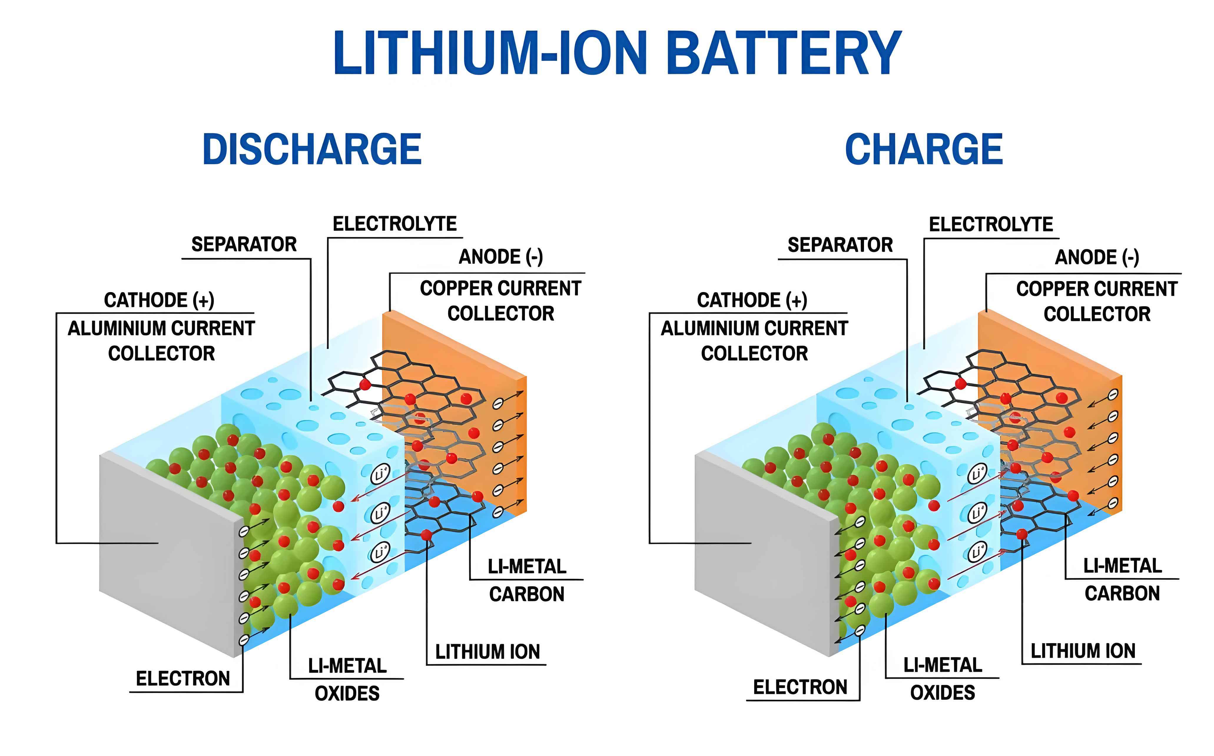
The dominance of the li ion battery in automotive applications is underpinned by a compelling set of advantages. Its superior energy density translates to longer driving ranges, while its impressive cycle life ensures durability over the vehicle’s lifetime. Unlike some older battery chemistries, li ion batteries exhibit a low self-discharge rate and minimal memory effect, simplifying operational management. Furthermore, they operate effectively across a wide temperature spectrum and offer a favorable balance of cost and performance. Structurally, a typical li ion cell comprises a positive cathode (often a lithium metal oxide like NMC or LFP), a negative graphite anode, a porous separator that prevents electrical shorting, and a lithium-salt electrolyte that facilitates ion transport. These components are housed within standardized formats such as cylindrical, prismatic, or pouch cells, with cylindrical cells being particularly prevalent in many EV battery module designs due to their mechanical robustness and efficient packing.
Equivalent Circuit Model Selection
Modeling the electrochemical processes within a li ion battery can be approached from multiple angles. While electrochemical models offer deep physical insight and neural network models provide black-box adaptability, Equivalent Circuit Models are favored for BMS applications due to their intuitive structure, moderate computational load, and sufficient accuracy for real-time control. An ECM represents the battery’s electrical behavior using a network of passive components like resistors, capacitors, and voltage sources. The complexity of the model can be scaled based on the required accuracy and available computational resources.
| Model Type | Circuit Diagram | Governing Equation(s) | Advantages | Disadvantages |
|---|---|---|---|---|
| Rint (Internal Resistance) Model | Voltage Source (OCV) in series with Resistor (R0) | $$U = U_{OCV} – I R_0$$ | Extremely simple, minimal computation. | Neglects polarization dynamics; highly inaccurate for dynamic currents. |
| Thevenin (1st Order RC) Model | Rint model + one RC parallel branch (R1, C1). | $$U = U_{OCV} – I R_0 – U_1$$, where $$U_1$$ is the voltage across the RC branch. | Captures basic polarization; good balance of simplicity and dynamic accuracy. | May be insufficient for capturing both fast and slow polarization dynamics, especially under wide temperature or aging conditions. |
| Second-Order RC Model | Rint model + two RC parallel branches (R1,C1 and R2,C2). | $$U = U_{OCV} – I R_0 – U_1 – U_2$$ | Accurately models both electrochemical and concentration polarization; widely regarded as an optimal trade-off for BMS use. | More parameters to identify; slightly higher computational cost than 1st order model. |
For this study, the second-order RC model is selected. Its architecture allows for the simultaneous representation of three critical physical phenomena: the instantaneous ohmic loss (via R0), the faster electrochemical polarization (via R1-C1), and the slower concentration polarization or diffusion effects (via R2-C2). This makes it significantly more accurate than simpler models, particularly under the high-current, transient conditions typical of automotive drive cycles. As microprocessor capabilities continue to advance, the computational burden of this model is no longer a limiting factor for real-time implementation in modern BMS hardware.
The electrical behavior of the second-order RC model for the li ion battery is governed by Kirchhoff’s laws. The terminal voltage $U$ is given by:
$$U = U_{OC} – I R_0 – U_1 – U_2$$
where $U_{OC}$ is the open-circuit voltage (a function of SOC and temperature), $I$ is the load current (positive for discharge), $R_0$ is the ohmic internal resistance, and $U_1$, $U_2$ are the voltages across the two polarization RC branches. The dynamics of the polarization voltages are described by:
$$\tau_1 \frac{dU_1}{dt} + U_1 = I R_1$$
$$\tau_2 \frac{dU_2}{dt} + U_2 = I R_2$$
where $\tau_1 = R_1 C_1$ and $\tau_2 = R_2 C_2$ are the time constants of the two polarization processes. For digital implementation in a BMS, these continuous-time equations are discretized. Using a zero-order hold (ZOH) assumption for the input current $I$ with a sampling period $T$, the discrete-time state-space representation is:
$$U_1(k+1) = e^{-T/\tau_1} U_1(k) + R_1 (1 – e^{-T/\tau_1}) I(k)$$
$$U_2(k+1) = e^{-T/\tau_2} U_2(k) + R_2 (1 – e^{-T/\tau_2}) I(k)$$
$$U(k+1) = U_{OC}(k+1) – I(k) R_0 – U_1(k+1) – U_2(k+1)$$
This formulation allows for the recursive prediction of the li ion battery terminal voltage based on the measured current and the identified model parameters.
Experimental Parameter Identification
The fidelity of the li ion battery model is entirely dependent on the accuracy of its parameters: $U_{OC}(SOC)$, $R_0(SOC)$, $R_1(SOC)$, $C_1(SOC)$, $R_2(SOC)$, and $C_2(SOC)$. These parameters are not constants; they vary significantly with the battery’s state of charge (SOC), temperature, and state of health (SOH). Therefore, a systematic experimental procedure is required to identify them as functions of SOC under controlled conditions.
The test subject was a commercially available 19 Ah ternary (NMC) cylindrical li ion battery with a nominal voltage of 3.7V and charge/discharge cut-off voltages of 4.1V and 2.8V, respectively. A high-precision battery test system was used to apply controlled current profiles and record voltage and current data. The cornerstone of the parameter identification process is the Hybrid Pulse Power Characterization (HPPC) test, a standardized profile designed to excite the battery’s dynamic response across its entire SOC range.
HPPC Test Procedure:
- The li ion battery is fully charged and then rested for a prolonged period (e.g., 12 hours) to ensure complete relaxation of all polarization effects, establishing a true equilibrium state.
- Starting from a high SOC (e.g., 90%), a sequence of pulses is applied at discrete SOC points (typically 9 or 10 points from 90% to 10% SOC). The sequence at each point is:
- Discharge Pulse: A 10-second discharge pulse at a high rate (e.g., 1C or specified power level).
- Rest Period: A 40-second rest.
- Charge Pulse: A 10-second charge pulse at a lower rate (e.g., 0.75C).
- Between each pulse sequence, a 1C constant current discharge is applied for a fixed duration (e.g., 6 minutes) to deplete the li ion battery to the next target SOC point, followed by a 1-hour rest period for relaxation.
This process is repeated until the lower voltage limit is reached.
Parameter Extraction from HPPC Data:
The analysis of the HPPC voltage response yields all necessary parameters. The key is to isolate sections of the response corresponding to specific model behaviors.
1. Open-Circuit Voltage (OCV) Identification:
After the long 1-hour rest period, the polarization voltages have fully decayed ($U_1 \approx 0$, $U_2 \approx 0$). At this equilibrium point, the terminal voltage equals the OCV. Therefore, the voltage measured at the end of each long rest period is recorded as the OCV for that corresponding SOC. A table of SOC-OCV pairs is constructed.
$$U_{OC}(SOC_i) = U_{terminal}(t_{end\_of\_rest})$$
| SOC | 0.9 | 0.8 | 0.7 | 0.6 | 0.5 | 0.4 | 0.3 | 0.2 | 0.1 |
|---|---|---|---|---|---|---|---|---|---|
| OCV (V) | 3.979 | 3.887 | 3.763 | 3.729 | 3.677 | 3.602 | 3.567 | 3.566 | 3.511 |
2. Ohmic Resistance ($R_0$) Identification:
At the instant a current pulse is applied (or removed), the polarization capacitors behave as short circuits because their voltage cannot change instantaneously. Therefore, the immediate jump or drop in terminal voltage is solely due to the ohmic resistance. For a discharge pulse starting at time $t_1$, $R_0$ is calculated as:
$$R_0(SOC) = \frac{|U(t_1^-) – U(t_1^+)|}{|I_{pulse}|}$$
where $U(t_1^-)$ is the voltage just before the pulse and $U(t_1^+)$ is the voltage just after the current step.
3. Polarization Parameters ($R_1, C_1, R_2, C_2$) Identification:
This involves analyzing the relaxation voltage curve after a pulse (zero-input response) and the voltage curve during a pulse (zero-state response). The relaxation voltage $U_{relax}(t)$ after a pulse ends at $t_2$ follows a double-exponential decay:
$$U_{relax}(t) = U_{OC} + A_1 e^{-(t-t_2)/\tau_1} + A_2 e^{-(t-t_2)/\tau_2}$$
By performing a non-linear curve fit (e.g., using MATLAB’s `fit` function or a least-squares algorithm) on the measured relaxation data, the amplitudes $A_1$, $A_2$ and time constants $\tau_1$, $\tau_2$ are obtained for each SOC point.
Subsequently, the zero-state response during the constant current pulse is analyzed. The governing equation for the terminal voltage during the pulse is:
$$U(t) = U_{OC} – I R_0 – I R_1 (1 – e^{-t/\tau_1}) – I R_2 (1 – e^{-t/\tau_2})$$
Since $U_{OC}$, $I$, $R_0$, $\tau_1$, and $\tau_2$ are now known, the only unknowns are $R_1$ and $R_2$. These can be solved for by evaluating the equation at two points during the pulse or through another fitting procedure. Finally, the polarization capacitances are calculated from the time constants:
$$C_1 = \frac{\tau_1}{R_1}, \quad C_2 = \frac{\tau_2}{R_2}$$
The complete set of identified parameters for the li ion battery across the SOC range is summarized below:
| SOC | $R_0$ (mΩ) | $R_1$ (mΩ) | $C_1$ (F) | $\tau_1$ (s) | $R_2$ (mΩ) | $C_2$ (F) | $\tau_2$ (s) |
|---|---|---|---|---|---|---|---|
| 0.9 | 3.44 | 3.26 | 7936 | 25.69 | 5.73 | 122 | 0.64 |
| 0.8 | 3.25 | 3.59 | 9256 | 32.63 | 5.92 | 147 | 0.88 |
| 0.7 | 3.22 | 2.57 | 14685 | 37.46 | 6.45 | 161 | 1.04 |
| 0.6 | 3.16 | 3.75 | 10425 | 39.22 | 6.10 | 123 | 0.73 |
| 0.5 | 3.14 | 3.17 | 11975 | 46.96 | 6.22 | 139 | 0.87 |
| 0.4 | 3.25 | 3.24 | 11397 | 36.63 | 6.10 | 127 | 0.76 |
| 0.3 | 3.10 | 4.17 | 9543 | 40.65 | 6.15 | 105 | 0.64 |
| 0.2 | 4.61 | 4.70 | 9233 | 43.09 | 6.23 | 95 | 0.59 |
| 0.1 | 4.37 | 5.74 | 8846 | 50.03 | 6.72 | 105 | 0.69 |
Model Implementation and Validation in Simulink
With the parameters fully identified, a dynamic simulation model of the li ion battery was constructed on the MATLAB/Simulink platform. The model core implements the discretized state-space equations. Key functional blocks include:
- Parameter Lookup: The SOC-dependent parameters ($U_{OC}$, $R_0$, $R_1$, $C_1$, $R_2$, $C_2$) are stored in 1-D lookup tables indexed by the instantaneous SOC.
- SOC Estimator: A simple coulomb counting integrator is used for simulation purposes: $$SOC(t) = SOC_0 – \frac{1}{Q_{nom}} \int_0^t I(\tau) d\tau$$ where $Q_{nom}$ is the nominal battery capacity (19 Ah).
- State Update Block: Calculates $U_1(k+1)$ and $U_2(k+1)$ using the discrete-time equations.
- Voltage Output Block: Computes the terminal voltage $U(k+1)$.
- Data Logging & Validation: Records simulation outputs (voltage, SOC, power loss) for comparison with real test data.
The model’s accuracy was rigorously validated against two distinct experimental profiles not used in the parameter identification HPPC test itself. The validation metric is the terminal voltage error, defined as:
$$Error(t) = U_{sim}(t) – U_{exp}(t)$$
$$Error\,Rate(t) = \frac{U_{sim}(t) – U_{exp}(t)}{U_{exp}(t)} \times 100\%$$
Validation 1: Dynamic HPPC Profile.
The model was simulated with the full HPPC current profile as input. The simulated terminal voltage trajectory was compared against the experimentally measured voltage. The results show excellent congruence. The model accurately captures the instantaneous voltage drops due to $R_0$, the subsequent exponential relaxation due to the RC networks, and the steady-state levels. The calculated error rate remains tightly bounded within a band of ±1.5% throughout the entire profile, with the absolute error rate predominantly under 1%.
Validation 2: Constant 1C Discharge Profile.
A more strenuous test is a continuous constant-current (1C) discharge from full to empty. This profile stresses the model’s ability to track the steady decline in OCV and the evolving polarization effects as SOC changes. The comparison demonstrates that the second-order RC model for the li ion battery performs superbly. The simulated voltage curve closely follows the experimental one, accurately replicating the entire discharge plateau. The error rate analysis confirms this, showing an absolute error rate consistently below 2% for the vast majority of the discharge, only approaching 3% near the very end of discharge where nonlinearities increase.
The performance of the li ion battery model under these two validation scenarios conclusively proves its accuracy and robustness. The absolute voltage error rate being controlled within 3% under both highly dynamic (HPPC) and steady (1C discharge) operational conditions meets and exceeds typical engineering requirements for BMS algorithms. This level of accuracy is sufficient for reliable state-of-charge estimation, power prediction, and crucially, for serving as a high-fidelity reference model in model-based fault diagnosis schemes. In such diagnostic applications, discrepancies between the voltage predicted by this accurate model and the voltage measured from the real li ion battery can be effectively used to detect anomalies, incipient faults, or performance degradation, thereby enhancing the safety and reliability of the vehicle’s energy storage system.
In conclusion, the methodology presented—selecting a second-order RC equivalent circuit model, performing systematic HPPC testing for parameter identification across the SOC range, and implementing a discrete-time simulation model—provides a powerful and practical framework for modeling vehicle lithium-ion batteries. The validation results underscore that this model is capable of predicting li ion battery terminal voltage with high precision under diverse loading conditions. This work establishes a solid foundation for advanced BMS functions, contributing to the optimization and safe operation of electric vehicles. Future work may focus on extending the model to account for temperature dependencies and aging effects to create an even more comprehensive li ion battery management tool.