
In recent years, the rapid development of new energy vehicles has been driven by increasing demands for sustainable energy and environmental protection, particularly under the “dual-carbon” targets. As a core component of these vehicles, the power li-ion battery offers advantages such as high energy density, long cycle life, and environmental friendliness. To ensure reliability and safety during operation, the battery management system (BMS) must accurately estimate and predict the state of charge (SOC) of li-ion batteries in real-time. However, SOC estimation remains challenging due to the nonlinear and time-varying characteristics of li-ion batteries. This article addresses this issue by proposing a method based on the extended Kalman filter (EKF) algorithm for precise SOC estimation. I will first introduce a second-order RC equivalent circuit model for li-ion batteries, then discuss parameter identification techniques, and finally detail the EKF-based SOC estimation approach, supported by simulations and experimental validations.
The accurate estimation of SOC is crucial for optimizing the performance and lifespan of li-ion batteries. SOC is defined as the ratio of remaining capacity to rated capacity, expressed as:
$$SOC(t) = SOC(t_0) – \int_{t_0}^{t} \frac{\eta I}{Q_n} dt$$
where \( t \) is time, \( \eta \) is the coulombic efficiency (typically 1 for li-ion batteries), \( I \) is the current (positive for discharge, negative for charge), and \( Q_n \) is the rated capacity of the li-ion battery. Various methods exist for SOC estimation, but many suffer from limitations such as cumulative errors or high computational demands. The EKF algorithm, which linearizes nonlinear systems, offers a robust solution with high accuracy and convergence properties, making it suitable for real-time BMS applications.
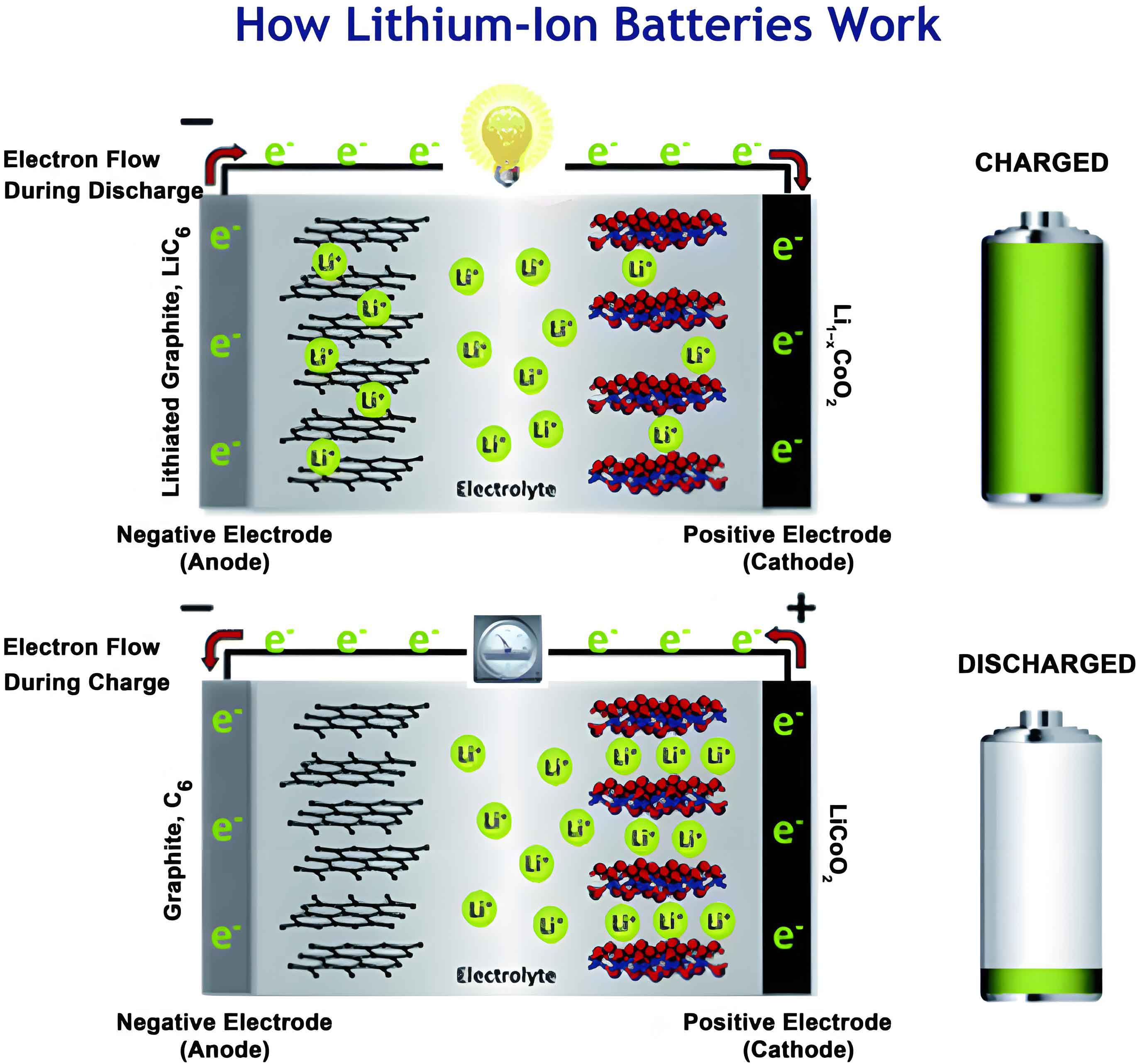
To model the li-ion battery, I adopt the second-order RC equivalent circuit model, which balances accuracy and computational complexity. This model includes an ohmic resistance \( R_0 \), two RC parallel branches representing electrochemical polarization (\( R_1, C_1 \)) and concentration polarization (\( R_2, C_2 \)), an open-circuit voltage (OCV) source \( U_{OC} \), and terminal voltage \( U_L \). The electrical behavior is described by Kirchhoff’s laws:
$$C_1 \frac{dU_1}{dt} = I – \frac{U_1}{R_1}$$
$$C_2 \frac{dU_2}{dt} = I – \frac{U_2}{R_2}$$
$$U_L = U_{OC} – U_1 – U_2 – I R_0$$
where \( U_1 \) and \( U_2 \) are polarization voltages. The OCV-SOC relationship is determined experimentally and fitted using a polynomial function. For a lithium iron phosphate (LiFePO4) soft-pack li-ion battery with a nominal capacity of 10 Ah, the OCV-SOC curve is approximated as:
$$U_{OC}(m) = 451m^9 – 2080m^8 + 4167m^7 – 4761m^6 + 3408m^5 – 1568m^4 + 455m^3 – 78.78m^2 + 7.56m + 2.91$$
where \( m \) represents SOC. This model forms the basis for parameter identification and SOC estimation of the li-ion battery.
Parameter identification is essential for refining the li-ion battery model. I compare two methods: offline identification using MATLAB/cftool toolbox and online identification via forgetting factor recursive least squares (FFRLS). Offline identification relies on hybrid pulse power characterization (HPPC) tests conducted at 25°C. The HPPC test involves applying pulse currents to the li-ion battery and measuring voltage responses. For example, the ohmic resistance \( R_0 \) is calculated from voltage drops during pulses:
$$R_0 = \frac{(U_A – U_B) + (U_D – U_C)}{2I}$$
where \( U_A, U_B, U_C, U_D \) are terminal voltages at specific points during the pulse. The polarization parameters \( R_1, C_1, R_2, C_2 \) are obtained by fitting the voltage relaxation curve to an exponential function:
$$y = a – b(1 – e^{-\frac{x}{c}}) – d(1 – e^{-\frac{x}{f}})$$
with \( y = U_L \), \( a = U_{OC} – I R_0 \), \( b = I R_1 \), \( c = R_1 C_1 \), \( d = I R_2 \), \( f = R_2 C_2 \), and \( x = t \). The offline identification results for the li-ion battery at different SOC levels are summarized in Table 1.
| SOC | \( R_0 \) (mΩ) | \( R_1 \) (mΩ) | \( R_2 \) (mΩ) | \( C_1 \) (F) | \( C_2 \) (F) |
|---|---|---|---|---|---|
| 0.1 | 3.20 | 1.17 | 3.23 | 5743.96 | 4334.37 |
| 0.2 | 2.97 | 5.46 | 3.35 | 3033.65 | 4179.11 |
| 0.3 | 2.50 | 3.35 | 3.48 | 3209.35 | 4024.15 |
| 0.4 | 2.30 | 4.09 | 5.19 | 3929.96 | 2697.50 |
| 0.5 | 2.16 | 3.83 | 2.16 | 4050.37 | 6487.49 |
| 0.6 | 2.04 | 3.61 | 3.31 | 4156.50 | 4227.05 |
| 0.7 | 1.96 | 1.10 | 3.61 | 14625.23 | 3985.28 |
| 0.8 | 1.86 | 3.86 | 2.89 | 4142.93 | 4619.88 |
| 0.9 | 1.78 | 3.46 | 3.09 | 5017.96 | 4533.68 |
| 1.0 | 1.95 | 2.55 | 3.51 | 2313.61 | 4145.14 |
However, offline methods only provide static parameters and may not capture dynamic changes in the li-ion battery during operation. To address this, I employ the FFRLS method for online parameter identification. The FFRLS algorithm updates parameters recursively to mitigate data saturation issues. The system output is expressed as:
$$y(k) = \varphi^T(k) \theta(k) + e(k)$$
where \( y(k) \) is the terminal voltage \( U_L(k) \), \( \varphi(k) \) is the data matrix, \( \theta(k) \) is the parameter vector, and \( e(k) \) is white noise. The recursive formulas are:
$$\hat{\theta}(k) = \hat{\theta}(k-1) + K(k) [y(k) – \varphi^T(k) \hat{\theta}(k-1)]$$
$$K(k) = \frac{P(k-1) \varphi(k)}{\lambda + \varphi^T(k) P(k-1) \varphi(k)}$$
$$P(k) = \frac{P(k-1) [E – K(k) \varphi^T(k)]}{\lambda}$$
where \( \lambda \) is the forgetting factor (0.95 < λ < 1), \( K(k) \) is the gain matrix, and \( P(k) \) is the error covariance matrix. For the second-order RC model of the li-ion battery, the discrete-time transfer function is derived using bilinear transform:
$$G(z^{-1}) = \frac{a_3 + a_4 z^{-1} + a_5 z^{-2}}{1 – a_1 z^{-1} – a_2 z^{-2}}$$
The coefficients \( a_1 \) to \( a_5 \) are related to the li-ion battery parameters \( R_0, R_1, C_1, R_2, C_2 \) through:
$$a_1 = \frac{2T^2 – 8\tau_1 \tau_2}{-(T^2 + 2T\tau_1 + 2T\tau_2 + 4\tau_1\tau_2)}$$
$$a_2 = \frac{T^2 – 2T\tau_1 – 2T\tau_2 + 4\tau_1\tau_2}{-(T^2 + 2T\tau_1 + 2T\tau_2 + 4\tau_1\tau_2)}$$
$$a_3 = \frac{T^2(R_0 + R_1 + R_2) + 2T(R_0\tau_1 + R_0\tau_2 + R_1\tau_2 + R_2\tau_1) + 4R_0\tau_1\tau_2}{-(T^2 + 2T\tau_1 + 2T\tau_2 + 4\tau_1\tau_2)}$$
$$a_4 = \frac{2T^2(R_0 + R_1 + R_2) – 8R_0\tau_1\tau_2}{-(T^2 + 2T\tau_1 + 2T\tau_2 + 4\tau_1\tau_2)}$$
$$a_5 = \frac{T^2(R_0 + R_1 + R_2) – 2T(R_0\tau_1 + R_0\tau_2 + R_1\tau_2 + R_2\tau_1) + 4R_0\tau_1\tau_2}{-(T^2 + 2T\tau_1 + 2T\tau_2 + 4\tau_1\tau_2)}$$
with time constants \( \tau_1 = R_1 C_1 \) and \( \tau_2 = R_2 C_2 \), and sampling time \( T \). The online identification results for the li-ion battery are shown in Table 2, demonstrating improved accuracy over offline methods.
| SOC | \( R_0 \) (mΩ) | \( R_1 \) (mΩ) | \( R_2 \) (mΩ) | \( C_1 \) (F) | \( C_2 \) (F) |
|---|---|---|---|---|---|
| 0.1 | 2.22 | 4.99 | 0.55 | 8024.74 | 1832.47 |
| 0.2 | 2.05 | 4.82 | 0.35 | 8297.78 | 2397.46 |
| 0.3 | 1.93 | 4.73 | 0.30 | 8370.51 | 2728.25 |
| 0.4 | 1.84 | 4.43 | 0.31 | 8555.39 | 3011.83 |
| 0.5 | 1.78 | 4.16 | 0.32 | 8992.82 | 3354.29 |
| 0.6 | 1.72 | 3.55 | 0.33 | 8971.54 | 3686.41 |
| 0.7 | 1.67 | 3.62 | 0.38 | 9649.81 | 3987.28 |
| 0.8 | 1.63 | 3.87 | 0.40 | 9121.60 | 4147.96 |
| 0.9 | 1.61 | 3.75 | 0.42 | 9102.63 | 4252.74 |
| 1.0 | 1.91 | 1.55 | 3.36 | 8775.94 | 1363.68 |
With the li-ion battery model and parameters established, I proceed to SOC estimation using the EKF algorithm. The EKF linearizes the nonlinear system of the li-ion battery for state estimation. The state vector is defined as \( x(k) = [SOC(k), U_1(k), U_2(k)]^T \), with input \( u(k) = I(k) \) and output \( y(k) = U_L(k) \). The discrete-time state and observation equations are:
$$x(k+1) = f(x(k), u(k)) + \omega(k)$$
$$y(k) = h(x(k), u(k)) + \nu(k)$$
where \( \omega(k) \) and \( \nu(k) \) are process and observation noises with covariances \( Q \) and \( R \), respectively. For the second-order RC model of the li-ion battery, these equations expand to:
$$\begin{bmatrix} SOC(k+1) \\ U_1(k+1) \\ U_2(k+1) \end{bmatrix} = \begin{bmatrix} 1 & 0 & 0 \\ 0 & e^{-\frac{\Delta t}{\tau_1}} & 0 \\ 0 & 0 & e^{-\frac{\Delta t}{\tau_2}} \end{bmatrix} \begin{bmatrix} SOC(k) \\ U_1(k) \\ U_2(k) \end{bmatrix} + \begin{bmatrix} -\frac{\Delta t}{Q_n} \\ (1 – e^{-\frac{\Delta t}{\tau_1}}) R_1 \\ (1 – e^{-\frac{\Delta t}{\tau_2}}) R_2 \end{bmatrix} I(k) + \begin{bmatrix} \omega_1(k) \\ \omega_2(k) \\ \omega_3(k) \end{bmatrix}$$
$$U_L(k) = \frac{\partial U_{OC}(SOC(k))}{\partial SOC(k)} \cdot SOC(k) – U_1(k) – U_2(k) – I(k) R_0 + \nu(k)$$
The EKF algorithm involves the following steps for the li-ion battery SOC estimation:
- Initialization: Set initial values for \( x(0) \), error covariance matrix \( P(0) \), and noise covariances \( Q \) and \( R \).
- State Prediction: Predict the next state using:
$$ \tilde{x}(k+1) = A(k) \hat{x}(k) + B(k) I(k) $$
where \( A(k) = \text{diag}(1, e^{-\frac{\Delta t}{\tau_1}}, e^{-\frac{\Delta t}{\tau_2}}) \) and \( B(k) = [-\frac{\Delta t}{Q_n}, (1 – e^{-\frac{\Delta t}{\tau_1}}) R_1, (1 – e^{-\frac{\Delta t}{\tau_2}}) R_2]^T \). - Error Covariance Prediction: Update the error covariance:
$$ \tilde{P}(k+1) = A(k) \hat{P}(k) A^T(k) + Q $$ - Kalman Gain Calculation: Compute the gain matrix:
$$ K(k+1) = \frac{\tilde{P}(k+1) C^T(k)}{C(k) \tilde{P}(k+1) C^T(k) + R} $$
with \( C(k) = \left[ \frac{\partial U_{OC}(SOC(k))}{\partial SOC(k)}, -1, -1 \right] \). - State Update: Correct the state estimate:
$$ \hat{x}(k+1) = \tilde{x}(k+1) + K(k+1) [y(k) – C(k) \tilde{x}(k+1) – D(k) I(k)] $$
where \( D(k) = -R_0 \). - Error Covariance Update: Adjust the error covariance:
$$ \hat{P}(k+1) = [E – K(k+1) C(k)] \tilde{P}(k+1) $$
These steps are repeated recursively to estimate the SOC of the li-ion battery in real-time. The EKF algorithm effectively handles nonlinearities and noise, making it ideal for li-ion battery applications.
To validate the proposed approach, I conducted simulations and experiments using a LiFePO4 soft-pack li-ion battery with a nominal capacity of 10 Ah. A BMS experimental platform was built to collect current and voltage data, with SOC computed in real-time and transmitted via CAN communication. The federal urban driving schedule (FUDS) was used as the test cycle to simulate realistic operating conditions for the li-ion battery. The FUDS current profile varies dynamically, challenging the SOC estimation accuracy. The model accuracy was first evaluated by comparing terminal voltage predictions from offline and online parameter identification methods. As shown in Table 3, the FFRLS-based online identification for the li-ion battery resulted in lower voltage errors compared to the offline method, confirming its superiority.
| Parameter Identification Method | Maximum Voltage Error (ΔU_L) | Average Voltage Error |
|---|---|---|
| Offline (MATLAB/cftool) | 0.168 V | 0.020 V |
| Online (FFRLS) | 0.07 V | 0.004 V |
The SOC estimation performance was then assessed using the EKF algorithm with online parameters for the li-ion battery. Two scenarios were tested: one with an initial SOC error (BMS SOC set to 0.95 vs. true SOC of 1.0) and another with accurate initial SOC (both set to 1.0). The results are summarized in Table 4. In both cases, the EKF algorithm demonstrated rapid convergence within 20 seconds and low estimation errors. For the li-ion battery with initial error, the maximum SOC error was 1.97%, with an average error of 0.0301%, while for the accurate initial case, the maximum error was 0.4108% and average error was 0.0773%. These errors comply with the GB/T 38661-2020 standard, which requires cumulative SOC estimation errors to be less than 5% for electric vehicle BMS.
| Initial SOC Condition | Convergence Time | Maximum SOC Error | Average SOC Error | Error Range After Convergence |
|---|---|---|---|---|
| BMS SOC = 0.95, True SOC = 1.0 | 20 s | 1.97% | 0.0301% | -1% to 2% |
| BMS SOC = 1.0, True SOC = 1.0 | 20 s | 0.4108% | 0.0773% | -0.5% to 0.3% |
The effectiveness of the EKF algorithm for li-ion battery SOC estimation is further highlighted by its ability to handle nonlinear dynamics and measurement noise. Compared to traditional methods like ampere-hour integration or open-circuit voltage, the EKF provides higher accuracy and robustness, essential for safe li-ion battery operation in electric vehicles. Moreover, the online parameter identification via FFRLS ensures that the li-ion battery model adapts to changing conditions, such as temperature variations or aging effects, though this study focused on room temperature without aging considerations. Future work could explore adaptive EKF versions or machine learning techniques to enhance li-ion battery SOC estimation under diverse operating scenarios.
In conclusion, this article presents a comprehensive method for SOC estimation of li-ion batteries using the EKF algorithm. By employing a second-order RC equivalent circuit model and online parameter identification with FFRLS, the li-ion battery model achieves high accuracy. The EKF algorithm effectively estimates SOC with rapid convergence and low errors, as validated through simulations and experiments under FUDS conditions. This approach meets industry standards and offers practical benefits for BMS in electric vehicles, contributing to the reliable and efficient use of li-ion batteries in sustainable transportation. The continuous improvement of such algorithms is vital for advancing li-ion battery technology and supporting global energy transition goals.