
The rapid integration of renewable energy sources into the power grid has underscored the critical role of energy storage systems (ESS). Among various technologies, the li ion battery stands out due to its high energy density, long cycle life, and relatively low environmental impact, making it a cornerstone for modern grid-scale storage. Ensuring the safety, reliability, and economic operation of these li ion battery systems falls upon the Battery Management System (BMS). A paramount parameter within the BMS is the State of Health (SOH), which quantifies the degree of degradation a battery has undergone relative to its fresh condition. Accurate SOH estimation is indispensable; it provides early warnings for potential failures, informs optimal maintenance schedules, and determines the right time for replacement, thereby maximizing the lifecycle value and safety of the storage asset.
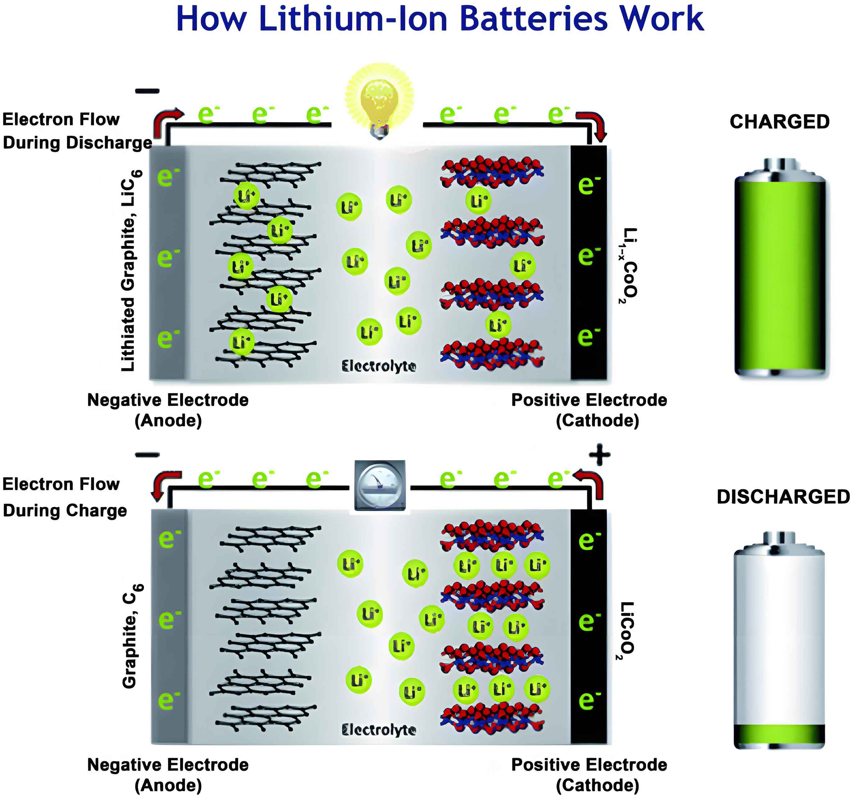
However, the SOH of a li ion battery is not directly measurable. It must be inferred from other operational data. Traditional model-based methods, which rely on equivalent circuit models coupled with filters like the Unscented Kalman Filter, often struggle with the complex, nonlinear electrochemical degradation processes inherent to li ion battery aging. The accuracy of these methods is heavily contingent on the precision of the underlying physical model, which is difficult to obtain universally. Consequently, data-driven methods, particularly those leveraging deep learning, have gained tremendous traction. These approaches learn the mapping between easily measurable operational parameters and the SOH directly from historical aging data, bypassing the need for explicit physical modeling.
Common deep learning architectures include Convolutional Neural Networks (CNN), adept at extracting spatial features from structured data, and Long Short-Term Memory (LSTM) networks, designed to capture temporal dependencies in sequential data. While previous studies have employed these networks individually or in simple combinations, they often fall short in fully exploiting the rich information embedded in li ion battery operational cycles. For instance, a standalone CNN might effectively process a single cycle’s data but ignore the crucial temporal trend across cycles. A standard LSTM might capture temporal patterns but could benefit from more potent feature representations of each cycle’s data as input.
To address these limitations, this work proposes a novel, hybrid data-driven framework that synergistically combines a Convolutional Neural Network (CNN) with a Bidirectional Long Short-Term Memory (Bi-LSTM) network for precise online SOH estimation of li ion battery. Our methodology is designed with practicality in mind: it uses readily available, easy-to-process features—average charging current, average discharging voltage, and average discharging temperature per cycle—eliminating the need for complex feature engineering or storing massive high-frequency datasets. The CNN layer acts as an automatic spatial feature extractor from the input grid data of each cycle. The subsequent Bi-LSTM layer then processes these enhanced feature sequences bidirectionally, capturing both past and future contextual dependencies in the aging trajectory. This two-stage, spatio-temporal analysis provides a more comprehensive understanding of li ion battery degradation, leading to superior estimation accuracy.
Theoretical Foundations of the Hybrid Model
The core innovation of our approach lies in the sequential and complementary application of CNN and Bi-LSTM. We first define the State of Health (SOH) from a capacity perspective, which is intuitive and directly related to the energy delivery capability of a li ion battery:
$$ SOH_i = \frac{Q_i}{Q_{nominal}} \times 100\% $$
where $SOH_i$ is the health state at cycle $i$, $Q_i$ is the discharge capacity measured at cycle $i$, and $Q_{nominal}$ is the rated capacity of the fresh li ion battery.
Convolutional Neural Network for Spatial Feature Extraction
The input for each charge-discharge cycle is formatted as a 1D grid (or sequence) of three features: $[I_{avg\_chg}, V_{avg\_dis}, T_{avg\_dis}]$. A one-dimensional CNN is exceptionally well-suited to process this structure. Its fundamental operation, the convolution, applies a set of learnable filters (kernels) to the input. For a 1D input vector $\mathbf{x}$ and a filter $\mathbf{w}$ of length $k$, the convolution operation at position $j$ is:
$$ (\mathbf{x} * \mathbf{w})[j] = \sum_{m=1}^{k} x_{[j+m]} \cdot w_{[m]} $$
where $*$ denotes the convolution operation. The CNN employs multiple such filters, each learning to detect different local patterns or relationships between the three input parameters. For example, one filter might learn to highlight a specific correlation between rising average discharge temperature and a particular range of average discharge voltage. The key advantages of CNN are:
- Local Feature Learning: It automatically extracts relevant spatial correlations within the feature set of a single cycle.
- Parameter Sharing: The same filter scans across the input, drastically reducing the number of trainable parameters compared to fully connected layers and improving computational efficiency.
- Hierarchical Representation: Stacking multiple convolutional layers allows the network to build increasingly abstract representations from the raw input data.
The output from the final CNN layer for each cycle is a transformed, high-dimensional feature vector that encapsulates the salient spatial characteristics of that cycle’s operational data, providing a more informative input for the sequential model.
Bidirectional LSTM for Temporal Dependency Modeling
The degradation of a li ion battery is a quintessential temporal process; the SOH at cycle $n$ is inherently dependent on the aging history of cycles $1$ to $n-1$. The Long Short-Term Memory (LSTM) network is designed to handle such long-term dependencies by introducing a gating mechanism. An LSTM unit maintains a cell state $\mathbf{C}_t$ (long-term memory) and a hidden state $\mathbf{h}_t$ (short-term memory/output). The operations at timestep $t$ are governed by three gates:
- Forget Gate ($\mathbf{f}_t$): Decides what information to discard from the cell state.
$$ \mathbf{f}_t = \sigma(\mathbf{W}_f \cdot [\mathbf{h}_{t-1}, \mathbf{x}_t] + \mathbf{b}_f) $$ - Input Gate ($\mathbf{i}_t$) and Candidate State ($\tilde{\mathbf{C}}_t$): Decide what new information to store and create a candidate update.
$$
\mathbf{i}_t = \sigma(\mathbf{W}_i \cdot [\mathbf{h}_{t-1}, \mathbf{x}_t] + \mathbf{b}_i) \\
\tilde{\mathbf{C}}_t = \tanh(\mathbf{W}_C \cdot [\mathbf{h}_{t-1}, \mathbf{x}_t] + \mathbf{b}_C)
$$ - Cell State Update: Combines the previous cell state and the new candidate information.
$$ \mathbf{C}_t = \mathbf{f}_t \odot \mathbf{C}_{t-1} + \mathbf{i}_t \odot \tilde{\mathbf{C}}_t $$ - Output Gate ($\mathbf{o}_t$): Decides what part of the cell state to output as the hidden state.
$$
\mathbf{o}_t = \sigma(\mathbf{W}_o \cdot [\mathbf{h}_{t-1}, \mathbf{x}_t] + \mathbf{b}_o) \\
\mathbf{h}_t = \mathbf{o}_t \odot \tanh(\mathbf{C}_t)
$$
where $\sigma$ is the sigmoid function, $\tanh$ is the hyperbolic tangent function, $\odot$ denotes the Hadamard (element-wise) product, $\mathbf{W}$ and $\mathbf{b}$ are weight matrices and bias vectors, $\mathbf{x}_t$ is the input at time $t$ (the CNN-extracted feature vector for cycle $t$), and $\mathbf{h}_{t-1}$ is the previous hidden state.
A standard LSTM processes sequences in the forward direction (past to future). However, the degradation context can be enriched by also considering the sequence from future to past. A Bidirectional LSTM (Bi-LSTM) achieves this by employing two separate LSTM layers: one processes the sequence forward ($\overrightarrow{\mathbf{h}_t}$), and the other processes it backward ($\overleftarrow{\mathbf{h}_t}$). The final output at each timestep is a concatenation or combination of both directional outputs:
$$ \mathbf{H}_t = g(\overrightarrow{\mathbf{h}_t}, \overleftarrow{\mathbf{h}_t}) $$
where $g$ is a concatenation or summation function. This bidirectional context allows the model to make SOH estimations for a given cycle based on the full historical and “future” (within the window) aging trend, leading to more robust and accurate predictions for the li ion battery.
Architecture and Implementation of the CNN-Bi-LSTM Model
The proposed hybrid model is structured as a sequential pipeline to maximize the strengths of both component networks. The overall architecture is designed to transform raw per-cycle measurements into a precise SOH estimate.
| Layer # | Layer Type | Key Parameters / Output Shape | Purpose |
|---|---|---|---|
| 1 | Input Layer | Shape: (batch_size, 1, 3) | Accepts raw input grid [I_avg_chg, V_avg_dis, T_avg_dis] per cycle. |
| 2 | 1D Convolutional | Filters: 256, Kernel: (1,3), Activation: ReLU | Initial spatial feature extraction. Learns 256 different local feature detectors. |
| 3 | 1D Convolutional | Filters: 128, Kernel: (1,3), Activation: ReLU | Further refines and abstracts the feature representation from Layer 2. |
| 4 | Flatten | Output: (batch_size, 128) | Converts the 3D feature map into a 1D feature vector for the sequential layer. |
| 5 | RepeatVector | n=30, Output: (batch_size, 30, 128) | Replicates the feature vector to create a sequence length of 30 for the LSTM input. |
| 6, 8, 9 | LSTM | Units: 100, Activation: tanh, Return_sequences: True | Stacked LSTM layers to learn complex, hierarchical temporal patterns in the aging data. |
| 7 | Dropout | Rate: 0.2 | Regularization layer to prevent overfitting by randomly dropping 20% of units. |
| 10 | Bidirectional LSTM | Wrapper(Bi-LSTM), Units: 128, Activation: ReLU | The core Bi-LSTM layer that processes sequences both forward and backward for comprehensive context. |
| 11 | Dense (Fully Connected) | Units: 100, Activation: ReLU | Further non-linear transformation and combination of the Bi-LSTM’s high-level features. |
| 12 | Dense (Output Layer) | Units: 1, Activation: Linear | Produces the final SOH estimation value for the target cycle. |
The training process follows a structured pipeline. First, data from publicly available li ion battery aging datasets (e.g., NASA) is preprocessed. The key input features—average charging current, average discharging voltage, and average discharging temperature—are calculated for each complete cycle. The target SOH values are computed using the capacity-based formula. The data is then normalized and split into training and testing sets. The model is trained by minimizing the Mean Absolute Error (MAE) between predictions and true SOH values using the Adam optimizer.
Experimental Validation and Performance Analysis
The model was implemented using TensorFlow/Keras in a Python environment. Validation was performed on the widely recognized NASA li ion battery aging dataset, specifically cells B0005 and B0006. These cells were cycled under controlled conditions until end-of-life, providing precise capacity fade curves essential for SOH validation.
| Feature Name | Description | Rationale for Selection |
|---|---|---|
| Average Charging Current ($I_{avg\_chg}$) | Mean current during the constant-current (CC) charging phase. | Reflects the standard charging protocol; variations can indicate internal resistance changes. |
| Average Discharging Voltage ($V_{avg\_dis}$) | Mean terminal voltage during the constant-current (CC) discharging phase. | Directly linked to the battery’s internal resistance and polarization; tends to drop with aging. |
| Average Discharging Temperature ($T_{avg\_dis}$) | Mean surface temperature during the CC discharging phase. | Indicates heat generation, which increases with degradation due to rising internal resistance. |
| Target: SOH | Computed as $Q_i / 2.0$ (Ah) * 100%. | The fundamental metric of li ion battery health and capacity retention. |
To objectively evaluate performance, we employ two standard regression metrics:
Mean Absolute Error (MAE): $$ MAE = \frac{1}{n}\sum_{i=1}^{n} |y_i – \hat{y}_i| $$
Root Mean Square Error (RMSE): $$ RMSE = \sqrt{\frac{1}{n}\sum_{i=1}^{n} (y_i – \hat{y}_i)^2} $$
where $n$ is the number of test samples, $y_i$ is the true SOH, and $\hat{y}_i$ is the estimated SOH. Lower values for both MAE and RMSE indicate higher estimation accuracy.
Our proposed CNN-Bi-LSTM model was benchmarked against two other prominent deep learning architectures: a standalone Bi-LSTM network (which processes the raw input features directly) and a CNN-LSTM network (which uses a forward-only LSTM after the CNN). This comparison isolates the contribution of the CNN’s spatial feature extraction and the Bi-LSTM’s bidirectional context.
| Battery Cell | Model | Mean Absolute Error (MAE) | Root Mean Square Error (RMSE) |
|---|---|---|---|
| B0005 | Bi-LSTM (Baseline) | 2.80 | 2.90 |
| CNN-LSTM | 1.11 | 1.38 | |
| Proposed CNN-Bi-LSTM | 1.04 | 1.19 | |
| B0006 | Bi-LSTM (Baseline) | 1.65 | 1.94 |
| CNN-LSTM | 1.42 | 1.71 | |
| Proposed CNN-Bi-LSTM | 1.07 | 1.32 |
The results are conclusive. On both li ion battery cells, the proposed CNN-Bi-LSTM model achieves the lowest MAE and RMSE, demonstrating superior estimation accuracy. The significant jump in performance from Bi-LSTM to CNN-LSTM (e.g., MAE drop from 2.80 to 1.11 for B0005) highlights the critical importance of the CNN layer for automatic spatial feature extraction from the simple input triple. The further, consistent improvement from CNN-LSTM to CNN-Bi-LSTM confirms the value of bidirectional temporal context for modeling li ion battery aging dynamics. The estimation errors for our model are consistently below 1.07 for MAE and 1.32 for RMSE, indicating a high degree of precision where most prediction errors are within a 2% band of the true SOH value.
Discussion and Implications for Energy Storage Systems
The successful development and validation of this CNN-Bi-LSTM model have several important implications for the management of grid-scale li ion battery energy storage. First and foremost, the model’s input requirements are pragmatic. BMS units in commercial ESS can easily log average current, voltage, and temperature per cycle without imposing significant data storage or transmission burdens. This makes the model highly deployable in real-world settings.
Secondly, the hybrid architecture offers a robust and generalizable solution. The CNN’s ability to distill meaningful features from raw data makes the model less sensitive to noise and minor variations in operating conditions. The Bi-LSTM’s comprehensive temporal analysis allows it to capture complex, non-linear degradation trajectories common to different li ion battery chemistries and usage patterns. This robustness is key for applications where operating profiles may not be perfectly uniform.
For system operators, integrating this SOH estimation capability enables a shift from reactive or schedule-based maintenance to predictive health management. By having a real-time, accurate view of each battery module’s health, operators can:
- Identify underperforming or rapidly degrading modules early, preventing cascading failures.
- Optimize the dispatch and cycling of assets to prolong the life of the overall system.
- Plan financials and logistics for replacement packs with greater accuracy.
- Enhance safety by monitoring for abnormal degradation signatures that could precede thermal events.
Future work will focus on enhancing the model’s generalizability across a wider array of li ion battery types, formats (cylindrical, pouch, prismatic), and diverse aging conditions (different temperatures, C-rates, depth-of-discharge profiles). Techniques like transfer learning and domain adaptation will be explored to allow a model pre-trained on laboratory data to be efficiently fine-tuned for a specific field-deployed li ion battery system with minimal new data. Furthermore, integrating this SOH estimator with prognostic models for Remaining Useful Life (RUL) prediction will provide a complete picture of the battery’s future state, maximizing the value and security of energy storage investments.
In conclusion, the fusion of CNN and Bi-LSTM presents a powerful, practical, and accurate framework for online SOH estimation of li ion battery. By effectively leveraging both spatial correlations within cycles and bidirectional temporal dependencies across cycles, this data-driven approach provides a reliable tool for ensuring the safe, efficient, and long-lasting operation of modern energy storage systems critical to our sustainable energy future.