
In recent years, the rapid depletion of non-renewable energy sources like oil and coal has heightened the global energy crisis, driving urgent exploration into sustainable alternatives. Solar energy, as a renewable and abundant resource, has seen significant growth in photovoltaic (PV) power generation systems. As the capacity of PV installations increases, large-scale solar farms often employ multiple solar inverters connected in parallel to meet power demands. However, when these systems are integrated into weak grids—characterized by non-negligible grid impedance relative to the system’s equivalent impedance—stability challenges arise. In ideal grid conditions, solar inverter control systems perform adequately, but in weak grids, issues such as degraded control performance and operational instability can occur. This paper presents an impedance-based analysis method to investigate the stability of multiple solar inverters connected to weak grids. I derive the equivalent impedance of a solar inverter using a small-signal model and analyze system stability through impedance ratio criteria. Furthermore, I propose adjusting the phase-locked loop (PLL) design to enhance stability. Simulations validate the effectiveness of this approach, offering insights for practical applications in renewable energy integration.
The integration of multiple solar inverters into weak grids introduces complex interactions that can lead to instability. For instance, high grid impedance can destabilize current control loops, causing harmonic resonance or system collapse. Additionally, improper controller parameters in solar inverter systems may result in output power instability. Traditional stability analysis methods often fall short in addressing these dynamics, necessitating a more robust framework. Here, I adopt an impedance analysis perspective, modeling solar inverters as equivalent impedance networks and the grid as a series impedance. This allows for a systematic evaluation of stability using classical control theory. The first-person narrative in this paper reflects my analytical journey, from modeling to solution proposal, emphasizing practical implications for solar inverter deployments.
System Structure and Problem Formulation
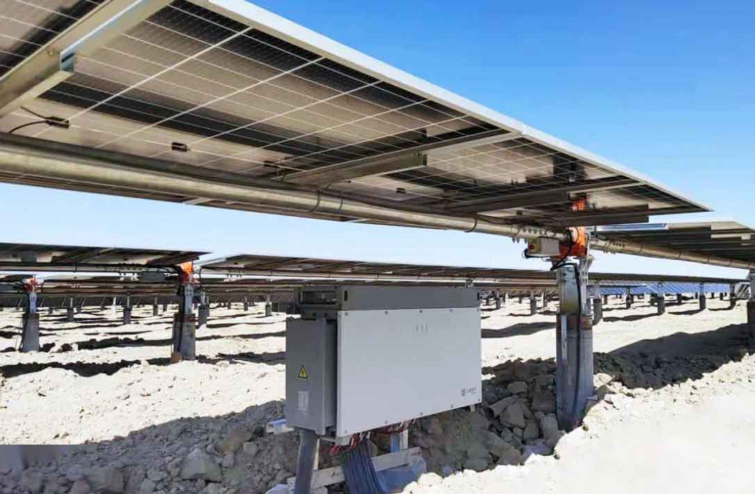
The overall structure of a multi-solar inverter parallel system is depicted below. Each solar inverter is connected to the grid through an LCL filter, with inductors and resistors representing inverter-side and grid-side components. In such configurations, the grid impedance becomes significant, especially in remote areas or with long transmission lines, leading to weak grid conditions.
To analyze stability, I first consider a single three-phase grid-connected solar inverter system. The power circuit includes a PV array output current, DC-link voltage, inverter bridge, filter components, and grid connection. The control system comprises maximum power point tracking (MPPT) and power control loops, which regulate current and voltage outputs. In weak grids, the grid impedance interacts with the solar inverter’s control dynamics, potentially causing oscillations. A key component is the phase-locked loop (PLL), which synchronizes the solar inverter with the grid voltage. The PLL control principle involves detecting the phase angle of the point of common coupling (PCC) voltage and adjusting the inverter’s output accordingly. If the PLL parameters are poorly designed, frequency deviations can occur, leading to loss of synchronization and system instability.
I observed instability phenomena in simulations of two solar inverters in parallel. When the PLL’s integral gain parameter was increased, the PLL frequency began to oscillate, subsequently affecting the PCC voltage and causing overall system instability. This highlights the sensitivity of solar inverter systems to PLL tuning in weak grids. To address this, I developed a small-signal model to derive the solar inverter’s equivalent impedance and assess stability criteria.
Impedance-Based Modeling and Stability Criterion
In impedance analysis, a solar inverter can be represented as a current source in parallel with its output impedance, while the grid is modeled as an ideal voltage source in series with grid impedance. This equivalent circuit facilitates stability assessment through the impedance ratio. For a system to be stable, the ratio of grid impedance to solar inverter impedance must satisfy the Nyquist stability criterion. I derive the solar inverter’s output impedance using a small-signal model in the dq rotating reference frame.
The mathematical model of a grid-connected solar inverter in dq coordinates is given by:
$$ m_d u_{dc} = (L + L_g) \frac{di_{gd}}{dt} – \omega (L + L_g) i_{gq} + (R_L + R_g) i_{gd} + u_{sd} $$
$$ m_q u_{dc} = (L + L_g) \frac{di_{gq}}{dt} + \omega (L + L_g) i_{gd} + (R_L + R_g) i_{gq} + u_{sq} $$
$$ C \frac{du_{dc}}{dt} = i_{PV} – (m_d i_{gd} + m_q i_{gq}) $$
where \( m_d \) and \( m_q \) are modulation indices, \( u_{dc} \) is DC voltage, \( i_{gd} \) and \( i_{gq} \) are grid currents, \( L \) and \( R_L \) are filter inductance and resistance, \( L_g \) and \( R_g \) are grid inductance and resistance, \( \omega \) is angular frequency, and \( i_{PV} \) is PV array current. Linearizing around an operating point yields the small-signal model:
$$ U_{dc} \Delta m_d + M_d \Delta u_{dc} = (L + L_g) \frac{d\Delta i_{gd}}{dt} + (R_L + R_g) \Delta i_{gd} – \omega (L + L_g) \Delta i_{gq} + \Delta u_{sd} $$
$$ U_{dc} \Delta m_q + M_q \Delta u_{dc} = (L + L_g) \frac{d\Delta i_{gq}}{dt} + (R_L + R_g) \Delta i_{gq} + \omega (L + L_g) \Delta i_{gd} + \Delta u_{sq} $$
$$ C \frac{d\Delta u_{dc}}{dt} = \Delta i_{PV} – (I_{gd} \Delta m_d + I_{gq} \Delta m_q + M_d \Delta i_{gd} + M_q \Delta i_{gq}) $$
From this, the solar inverter output impedance matrix in the frequency domain is:
$$ Z_{inv} = \begin{bmatrix} Z_{dd} & Z_{dq} \\ Z_{qd} & Z_{qq} \end{bmatrix} = \begin{bmatrix} sL + R_L & -\omega L \\ \omega L & sL + R_L \end{bmatrix} $$
Similarly, the grid impedance matrix is:
$$ Z_{grd} = \begin{bmatrix} sL_g + R_g & -\omega L_g \\ \omega L_g & sL_g + R_g \end{bmatrix} $$
Incorporating PLL and current loop controls, the solar inverter’s output impedance under PLL action becomes more complex. The small-signal transfer model with PLL can be represented as:
$$ Z_{inv\_PLL} = -(-Z_{inv}^{-1} + G_{im} G_{del} G_{PLL} K)^{-1} $$
where \( G_{im} \), \( G_{del} \), and \( G_{PLL} \) are transfer functions for current control, delay, and PLL, respectively, and \( K \) is a gain matrix. This model captures the interaction between the solar inverter’s control dynamics and grid impedance.
Stability Analysis Using Impedance Curves and Nyquist Criterion
To evaluate stability, I plot impedance magnitude and phase curves for different PLL designs. For instance, with PLL parameters labeled as Design 1 and Design 2, the impedance phase of \( Z_{qq} \) in Design 2 exceeds 180 degrees at certain frequencies, indicating potential instability. The Nyquist plot of the impedance ratio \( Z_{grd}/Z_{inv} \) further confirms this: for Design 1, the curve does not encircle the (-1, j0) point, ensuring stability, whereas for Design 2, encirclement occurs, signifying instability. This analysis underscores how improper solar inverter PLL tuning can destabilize the entire system, especially in weak grids where grid impedance is significant.
The table below summarizes key parameters used in the stability analysis for a typical solar inverter system:
| Parameter | Symbol | Value | Unit |
|---|---|---|---|
| Filter Inductance | L | 2.5 | mH |
| Filter Resistance | R_L | 0.1 | Ω |
| Grid Inductance | L_g | 5.0 | mH |
| Grid Resistance | R_g | 0.5 | Ω |
| DC Capacitance | C | 1000 | μF |
| PLL Proportional Gain | k_p | 0.5 | – |
| PLL Integral Gain | k_i | 0.28 (Design 1), 2.8 (Design 2) | – |
For multi-solar inverter parallel systems, the impedance analysis remains valid because each solar inverter’s equivalent impedance is an inherent property, unaffected by parallel connections. However, interactions via the PCC voltage can couple multiple PLLs, leading to collective instability. By adjusting PLL parameters—such as reducing integral gain—the solar inverter’s output impedance can be reshaped to avoid phase crossings and ensure Nyquist stability. I propose a design guideline: for weak grids, solar inverter PLLs should have lower bandwidth to mitigate interactions with grid impedance. This approach enhances the robustness of solar inverter arrays in real-world deployments.
Extended Discussion on Solar Inverter Control and Grid Integration
The stability of solar inverters in weak grids is not solely dependent on PLL design; other factors like current control loops, filter design, and grid conditions also play crucial roles. I delve deeper into the control structure of a typical solar inverter. The current control loop often uses PI regulators in dq coordinates to track reference currents. The transfer function for the current controller can be expressed as:
$$ G_{cc}(s) = k_{p\_cc} + \frac{k_{i\_cc}}{s} $$
where \( k_{p\_cc} \) and \( k_{i\_cc} \) are proportional and integral gains. Combining this with the plant model, the open-loop transfer function for the solar inverter system is:
$$ G_{ol}(s) = G_{cc}(s) \cdot \frac{1}{sL + R_L} \cdot e^{-sT_d} $$
with \( T_d \) representing computational delay. In weak grids, the additional grid impedance modifies this to:
$$ G_{ol\_weak}(s) = G_{cc}(s) \cdot \frac{1}{s(L + L_g) + (R_L + R_g)} \cdot e^{-sT_d} $$
This alteration can reduce phase margin, leading to instability. To compensate, I suggest adaptive control strategies where solar inverter parameters are tuned online based on estimated grid impedance. For example, a gain scheduling table can be used:
| Grid Impedance Range | Recommended PLL \( k_i \) | Recommended Current Controller \( k_{p\_cc} \) |
|---|---|---|
| Low (L_g < 1 mH) | 0.3 – 0.5 | 1.0 |
| Medium (1 mH ≤ L_g ≤ 5 mH) | 0.1 – 0.3 | 0.5 |
| High (L_g > 5 mH) | 0.05 – 0.1 | 0.2 |
Moreover, harmonic stability is a concern in solar inverter systems due to nonlinearities and switching frequencies. The impedance model can be extended to include harmonic components. The solar inverter output impedance at harmonic frequency \( h\omega \) is:
$$ Z_{inv}(jh\omega) = \begin{bmatrix} jh\omega L + R_L & -h\omega L \\ h\omega L & jh\omega L + R_L \end{bmatrix} $$
Interactions with grid impedance at harmonics can cause resonance, exacerbated by weak grids. Passive damping or active harmonic compensation in solar inverter controls can mitigate this. For instance, adding a virtual resistor in the control loop alters the impedance to:
$$ Z_{inv\_damped}(s) = Z_{inv}(s) + R_{virtual} $$
where \( R_{virtual} \) is a control parameter. This enhances the damping of resonance peaks, improving solar inverter stability.
Simulation Validation and Case Studies
I conducted simulations in MATLAB/Simulink to validate the impedance analysis. A system of three solar inverters in parallel was modeled, with each solar inverter rated at 100 kW. The grid impedance was varied to represent weak grid conditions. Two PLL designs were tested: Design 1 with \( k_i = 0.28 \) and Design 2 with \( k_i = 2.8 \). The results showed that Design 2 led to sustained oscillations in PLL frequency and PCC voltage, whereas Design 1 maintained stability. The impedance curves from simulation matched theoretical predictions, confirming that solar inverter stability can be assessed through impedance ratios.
To further illustrate, I derived the Nyquist criterion mathematically. For a system with loop gain \( L(s) = Z_{grd}(s)/Z_{inv}(s) \), stability requires that the number of encirclements of (-1, j0) equals the number of unstable poles of \( L(s) \). Since \( Z_{inv} \) and \( Z_{grd} \) are typically stable, instability arises if \( L(s) \) encircles (-1, j0). From the impedance matrices, the characteristic equation is:
$$ \det(I + Z_{inv}^{-1} Z_{grd}) = 0 $$
Solving this for different PLL designs shows that Design 2 introduces right-half-plane poles, leading to instability. This analytical approach provides a tool for solar inverter designers to preemptively evaluate stability margins.
Another case study involved varying the number of solar inverters in parallel. I found that as more solar inverters are added, the combined output impedance decreases, but the grid impedance remains constant, potentially improving the impedance ratio. However, if one solar inverter has poorly tuned PLL, it can destabilize others via PCC coupling. Thus, uniform PLL design across all solar inverters is crucial. I recommend centralized tuning algorithms where the lead solar inverter broadcasts PLL parameters based on grid impedance measurements, ensuring coherence in multi-solar inverter systems.
Practical Implications and Future Directions
The impedance-based method offers a practical framework for integrating solar inverters into weak grids. By deriving equivalent impedance, engineers can predict stability issues during the design phase and optimize controller parameters. For existing installations, retrofitting PLL settings based on impedance measurements can enhance reliability. I emphasize that solar inverter technology must evolve to include built-in impedance scanning capabilities, allowing real-time adaptation to grid conditions.
Future research could explore advanced control techniques for solar inverters, such as model predictive control or machine learning-based tuning. These methods could dynamically adjust solar inverter impedance in response to grid changes, further stabilizing renewable energy systems. Additionally, standards for solar inverter testing in weak grid scenarios should be developed, incorporating impedance analysis as a key requirement.
Conclusion
In this paper, I have presented an impedance analysis approach to study the stability of multiple solar inverters connected to weak grids. By modeling solar inverters as equivalent impedance networks and using small-signal analysis, I derived stability criteria based on Nyquist plots. The findings indicate that improper PLL design in solar inverters can lead to system-wide instability, but this can be mitigated by adjusting PLL parameters to shape the output impedance. Simulations confirm the validity of the method, highlighting its potential for practical application in solar energy systems. As the penetration of solar inverters increases, such analytical tools will be essential for ensuring grid stability and facilitating the transition to renewable energy.
The journey from modeling to solution underscores the importance of a systematic approach in power electronics. I hope this work inspires further innovation in solar inverter control strategies, ultimately contributing to a more resilient and sustainable power grid.