
Under the background of “dual carbon”, renewable energy represented by wind power has developed rapidly in recent years. However, the randomness and volatility of its output have posed challenges to the safe and stable operation of the power system. Therefore, measures need to be taken to improve the fluctuation of wind power grid connection points. The development of energy storage technology provides technical support for this. The composite energy storage system composed of lithium batteries and supercapacitors has the characteristics of flexible charging and discharging, fast response, and obvious advantages when applied to suppress wind power fluctuations. However, considering cost factors, further exploration is needed to optimize the capacity configuration of both while meeting demand.
The existing research on capacity allocation mainly includes simulation analysis method and optimization model method. The simulation analysis method uses filtering algorithms and frequency domain analysis to determine the capacity configuration of energy storage systems, proposes a power allocation strategy based on low-pass filtering, and determines the cutoff frequency through spectral analysis; Allocate energy storage power based on high pass filtering, and adaptively determine the cutoff frequency through the energy storage SOC state; Combining the Wiener stochastic process, a first-order Butterworth based energy storage power allocation strategy is proposed, and the energy storage capacity is configured based on the probability distribution and confidence interval of wind power variation. However, there is phase lag in the process of smoothing wind power through first-order low/high pass filtering, which leads to trend components in the allocated energy storage power and increases the allocation of energy storage capacity; Based on a composite energy storage system to suppress power fluctuations, a fixed window sliding average method is used to smooth wind power, and internal power is allocated in combination with wavelet packets. Then, the wavelet packet boundary point is determined through spectral analysis; Adopting adaptive sliding average method to smooth wind power, then allocating internal power based on empirical mode decomposition, and determining the boundary point with the least modal mixing; Using wavelet packet decomposition of wind power, the low-frequency power is connected to the grid, and the frequency band boundary point is determined with the minimum annual cost. The above research analyzed the configuration of energy storage capacity from different perspectives, but did not consider the impact of periods with large wind power fluctuations on the overall smoothing effect during the smoothing process, resulting in poor tracking ability of grid connected power on wind power during other periods with small fluctuations, and increased energy storage capacity configuration. The optimization model method considers energy storage costs, benefits, etc., and constructs optimization models with different objective functions to solve the energy storage capacity configuration scheme. A composite energy storage capacity optimization configuration model was constructed that takes into account the assessment of grid connected power exceeding limits and the penalty for SOC exceeding limits, and an improved particle swarm optimization algorithm was used to solve the problem; Referring to the grid connection standards, the grid connection components are determined through rule constraints, and then a composite energy storage output strategy and capacity configuration model are established, and an improved genetic algorithm is proposed for solution; Considering the investment and operating costs of the energy storage system, a capacity allocation model with the minimum annual average cost of composite energy storage was established. Chaos algorithm was used to solve the problem. The optimization model method was used to consider factors such as cost and benefit, making the obtained capacity allocation plan more economically convincing. However, the allocation results are related to the weights of different parts of the objective function at different levels. In addition, the wind power is smoothed through wavelet packet decomposition and empirical mode decomposition, and then a capacity configuration model is constructed with the minimum annual cost to solve the configuration scheme. However, during the smoothing process, the overall smoothing effect and local wind power tracking effect are also not taken into account, making it impossible to obtain a better composite energy storage total power.
In this regard, this article separates the total power allocation of composite energy storage and the internal power decoupling process in the capacity configuration process. Firstly, a composite energy storage total power allocation strategy is obtained using the adaptive time window wavelet packet method, which can adaptively plan the filtering time window to balance the smooth overall wind power and local wind power tracking ability, reducing the burden on the composite energy storage system; Secondly, based on SG filtering to decouple internal power, a composite energy storage life cycle cost-benefit model is constructed with SG filtering parameters as decision variables and the goal of maximizing net benefits, ensuring the economic feasibility of the configuration scheme; And an improved Harris Eagle algorithm solution model is proposed, which enhances the information sharing of dominant individuals by introducing an elite level strategy. A nonlinear energy function and Gaussian random walk strategy are proposed to balance the search ability at each stage and avoid falling into local optima. Finally, the effectiveness of the proposed strategy and the efficiency of the solving algorithm were verified based on actual wind farm data.
1.Composite energy storage total power allocation strategy based on adaptive time window wavelet packet
Using the national grid connection standard as a constraint, the wavelet packet decomposition level is adaptively determined to ensure that the smoothed grid connection power of a certain wind power data length meets the requirements and can track wind power well. Then, in order to control the impact of large wind power fluctuations on the smoothing effect in a small range, the time window concept and adaptive filtering time window planning method are proposed. By sliding the time window, the composite energy storage total power allocation can be achieved.
1.1 Determination of adaptive wavelet packet decomposition layers based on grid connection standards
The number of wavelet packet decomposition layers corresponds to the degree of signal decomposition and is related to the smoothness of wind power. Based on the national grid connection standard, the minimum number of wavelet packet decomposition layers that meet the smoothing requirements is determined. Firstly, initialize the decomposition level n to 0; Take the wind power Pw as the initial grid connection power Pn, and determine whether it meets the national grid connection standards. If it meets the requirements, it will be connected to the grid. Otherwise, the wind power will be decomposed into n-layer wavelet packets based on db6 wavelet, and the power components of 2n frequency bands in n-layer will be reconstructed. Then, the low-frequency power components Pn, 0 will be taken as the grid connected power, and the sum of the power components of the other frequency bands ∑ Pn, i, i=1,2 2 ^ (n-1) as the total power of composite energy storage.
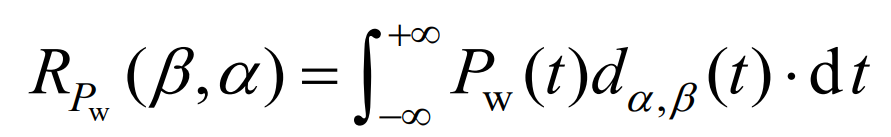
The process of wind power decomposition in this process is shown in equation (1).
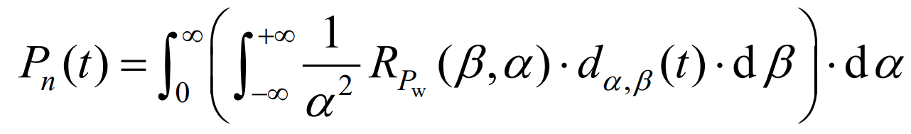
The power reconstruction process is shown in equation (2).
Among them,
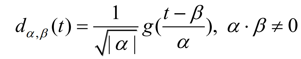
In the equation, α Is the scale factor; β Is the movement factor; Pw (t) and Pn (t) are the wind power and reconstructed power at time t; RPw( β,α) Decompose the energy of wind power onto the base coordinate axis; D α,β (t) For wavelet basis.
Determine whether Pn and 0 meet the national grid connection standards. If they meet the requirements, determine the number of wavelet packet decomposition layers as n. Otherwise, increase the number of wavelet packet decomposition layers n=n+1 and repeat the above process again.
The process of determining the number of layers for adaptive wavelet packet decomposition is described as follows:
1) Read the wind power data Pw and set the initial grid connected power Pn, 0=Pw; Make the number of decomposition layers n=0.
2) If Pn, 0 does not meet the requirements for grid connected power fluctuations at two time scales of 1 minute and 10 minute.
① Let n=n+1;
② Perform n-layer wavelet packet decomposition;
③ Reconstruct the power components of 2 ^ n frequency bands in the nth layer;
④ Let Pn, 0 be the reconstructed low-frequency power component, and add the sum of high-frequency power 1, ∑ Pn, i, i=1,2 2 ^ (n-1) as the total power of composite energy storage.
1.2 Determination of adaptive filtering time window considering wind power fluctuation characteristics
Under a certain wind power data length, the optimal composite energy storage total power can be obtained through the method in Section 1.1. The analysis is shown in Appendix A. However, as the data length increases, the overall smoothing effect is determined by the period of maximum fluctuation, resulting in poor tracking of wind power by the smoothed grid connected power in other periods, increasing the burden on the composite energy storage system. The analysis is shown in Appendix B. In order to ensure that the smoothed grid connected power meets the grid connected standards and has good local wind power tracking ability, and reduce the composite energy storage burden, an adaptive filtering time window planning method is proposed based on Section 1.1.
The length of the wind power Pw data is Lw, and the filtering time window is Tw (u). Firstly, initialize the filtering time window Tw (u) to Lw, and adaptively determine the number of wavelet packet decomposition layers n within the Tw (u) time window. Take the low-frequency power component Pn, 0 [Tw (u)] reconstructed from the nth layer for grid connection. And then with Δ The Tw (u) sliding time window is used to achieve smooth overall wind power and determine whether the overall grid connected power Pn, 0 [Tw (u), Lw] meets the grid connected standards. If satisfied, reduce the time window Tw (u)=Tw (u)+ Δ Tw (u), then repeat the above process; If not, then determine the filtering time window as Tw (u)=Tw (u)- Δ Tw (u), and take the corresponding Pn, 0 [Tw (u), Lw] under the Tw (u) time window as the grid connected power. The difference between the grid connected power and wind power is borne by the composite energy storage system, as shown in equation (4).
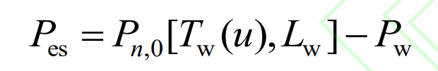
In the formula, Pes is the total power of composite energy storage; Pn, 0 [Tw (u), Lw] is the grid connected power smoothed by the Tw (u) time window.
During this process, when Tw (u) is 1h-24h, Δ When Tw is taken as 1 hour and Tw (u) is between 10 minutes and 1 hour, Δ Tw is taken for 10 minutes.
The process of adaptive time window planning and planning is described as follows:
1) Read the wind power data Pw and data length Lw; Make the filtering time window Tw (u)=Lw.
2) Based on adaptive wavelet packet decomposition, the grid connected power under Tw (u) is obtained, Pn, 0 [Tw (u), Lw].
3) If Pn, 0 [Tw (u), Lw] meets the requirements for grid connected power fluctuation rate at two time scales of 1 minute and 10 minute.
① Make Tw (u)=Tw (u)- Δ Tw (u);
② Obtain grid connected power Pn, 0 [Tw (u)] based on adaptive determination of wavelet packet decomposition within the Tw (u) time window;
4) If Pn, 0 [Tw (u), Lw] does not meet the requirements for grid connected power fluctuation rate at the time scales of 1 minute and 10 minutes.
① Then make Tw (u)=Tw (u)+ Δ Tw (u);
② Take Pn, 0 [Tw (u), Lw] as the grid connected power;
③ Take Pn, 0 [Tw (u), Lw] – Pw as the total power of composite energy storage.
2.Optimization and Configuration Model of Composite Energy Storage System Capacity Based on SG Filter Decoupling
After the total power allocation of composite energy storage is completed, further internal power allocation is required. Due to the effective ability of SG filtering to maintain the main characteristics of the signal and remove high-frequency components, this paper uses this as the basis for internal power decoupling and capacity configuration of the algorithm. Considering that the decoupling effect is related to SG filtering parameters, and in order to balance economic efficiency, a composite energy storage life cycle cost-benefit model is constructed using SG filtering parameters as decision variables. With the goal of maximizing net benefits, the improved Harris Eagle algorithm is used to solve the capacity allocation scheme.
2.1 Internal power decoupling strategy based on SG filtering
The core of SG filtering is to perform weighted filtering on the data within the window, and the weights are obtained by least squares fitting on a given high-order polynomial. Using time t0 as the center, perform k-1 polynomial fitting on the total power of composite energy storage within a window of 2n0+1 length, as shown in equation (5):
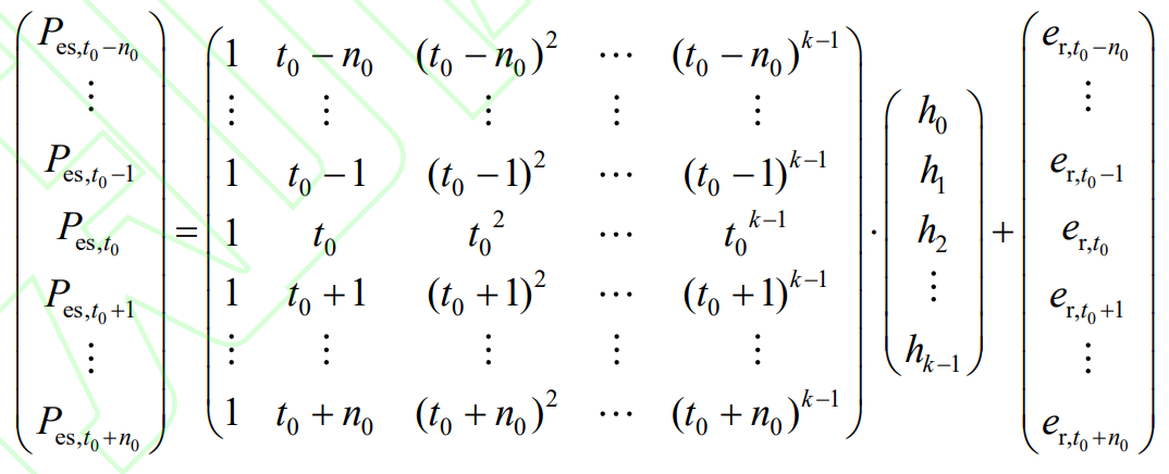
Record as,
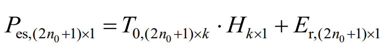
In the formula, h is the polynomial fitting coefficient; E is the fitting error.
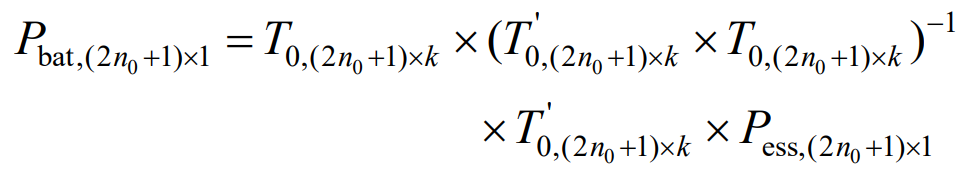
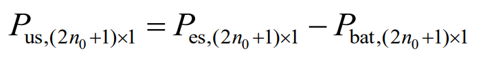
This process constructs a function of the sum of squares of errors between the composite energy storage power data points and the fitted power curve within the window. With the goal of minimizing the sum of squares of errors, the polynomial fitting coefficient H=(T’0 · T0) ^ -1 · T’0 · Pes, (2n0+1) x1, is calculated by calculating the partial derivative. Furthermore, it is worth noting that it is necessary to satisfy 2n0+1>k to ensure that equation (5) has a solution. Furthermore, the fitting power, also known as the lithium battery power, is obtained as shown in equation (7).
The supercapacitor bears the high-frequency part of the power command, represented by:
2.2 Capacity optimization model for composite energy storage system
2.2.1 Capacity Configuration Model
The principle of energy storage power configuration is to meet the maximum power demand during the operating cycle. Represented as:
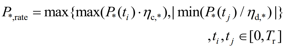
In the formula, P * and rate represent the energy storage power configuration; P * is the energy storage power command; η c. * η d. * Respectively refer to the energy storage charging and discharge efficiency* Representing lithium batteries or supercapacitors; Tr is the simulation cycle.
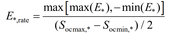
The principle of energy storage capacity configuration is to avoid operating under overcharging and discharging. Assuming that the initial state of the energy storage SOC is 0.5, the capacity configuration can be obtained based on the cumulative energy curve, expressed as:
Among them,
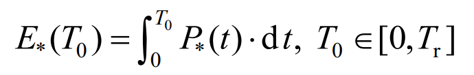
In the formula, E *, rate represents the energy storage capacity configuration; E * is the accumulated calming energy; Socmax, *, Socmin, * are the upper and lower limits of the state of charge during energy storage operation.
2.2.2 Quantitative Model for Composite Energy Storage Life
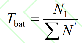
The cycle life of lithium batteries is a function of the depth of discharge (DOD), and the test data provided by engineering experiments is generally the maximum number of cycles under a fixed DOD. However, during the process of suppressing fluctuations in lithium batteries, DOD changes in real time. Therefore, this article uses the rain flow counting method to calculate the equivalent charging and discharging cycles under different DODs. Based on the relationship curve between DOD and cycle life and the equivalent cycle life method, the corresponding cycle times N of different DODs are converted to the equivalent cycle times N ‘under DOD=1 and summed up. Then, based on the comparison with the maximum cycle times N1 under DOD=1, the actual operating life Tbat of the lithium battery is obtained, as shown in equation (12).
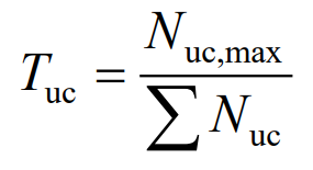
The lifespan of supercapacitors is relatively long and not significantly related to DOD. The main factor affecting their lifespan is the number of charges and discharges. The actual operating lifespan of supercapacitors can be calculated based on the actual number of charges and discharges and the maximum number of charges and discharges Nuc, max, as shown in equation (13). Among them, the transition of supercapacitors from charging to discharging and then to charging is recorded as charging and discharging once, i.e. Nuc=1.
2.2.3 Objective Function and Constraints
Considering the costs and benefits generated during the life cycle of the load energy storage system, including initial investment costs, replacement costs, auxiliary equipment costs, operation and maintenance costs, scrap disposal costs and recovery residual values, as well as the benefits of delayed grid connection channels, the objective function is constructed to maximize net benefits, as shown in equation (14).

Among them, Ctz is the initial investment cost, including the power investment cost and capacity investment cost of the composite energy storage system, expressed as:
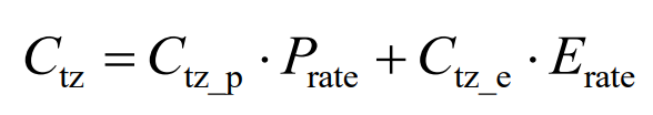
In the equation, Ctz_ P is the investment cost per unit power, Ctz_ E is the investment cost per unit capacity.
Cfz is the cost of auxiliary equipment, including the investment cost of auxiliary supporting equipment for the composite energy storage system, expressed as:
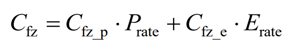
In the equation, Cfz_ P is the auxiliary cost per unit power; Cfz_ E is the auxiliary cost per unit capacity.
Cyw represents the cost of operation and maintenance, including the cost invested to ensure the normal operation of the composite energy storage system. It consists of a fixed portion (related to Prate) and a variable portion (related to charging and discharging capacity), expressed as:
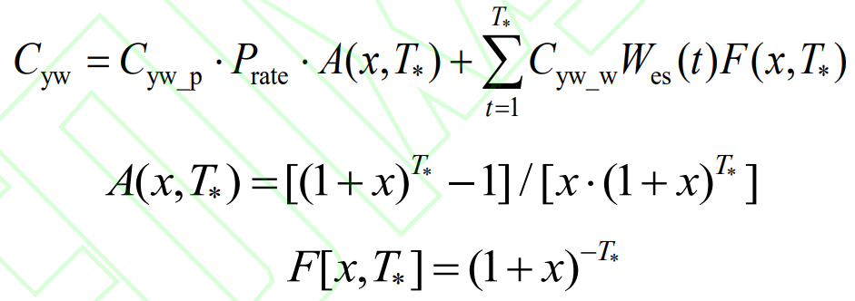
In the equation, Cyw_ P is the unit power operation and maintenance cost; Cyw_ W is the unit charge and discharge electricity operation and maintenance cost; Wes is the charging and discharging capacity during the energy storage life cycle; A (x, T *) is the present value coefficient of equal distribution; F [x, T *] is the one-time cash payment coefficient; T * is the life cycle, in years; X is the discount rate, taken as 0.1.
Cgx represents the replacement cost, including the cost incurred during the life cycle of the composite energy storage system due to component loss, aging, or the need to replace components that meet scrap standards, expressed as:
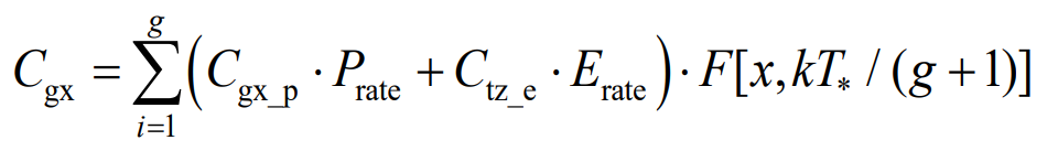
In the equation, Cgx_ P is the unit power update cost; G is the number of replacement times for energy storage components, and k is the number of replacement years.
Ccl is the cost of scrap disposal, including the cost required to dispose of composite energy storage system components when they are scrapped, expressed as:
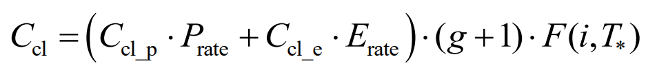
In the equation, Ccl_ P is the cost of scrapping per unit power; Ccl_ E is the cost of scrapping per unit capacity.
Chs is the residual value of recycling, including the benefits that can be obtained through recycling, utilization, etc. when the components of the composite energy storage system are scrapped, expressed as:
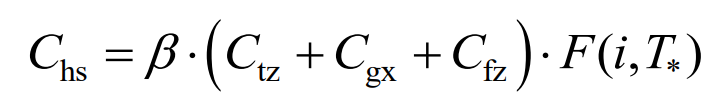
In the equation, β To recover the residual value rate, it is generally taken as 0.03-0.05.
Chj represents the benefits of delaying the construction of grid connection channels. Due to the fact that the capacity of wind farm grid connected channels is generally planned based on maximum output, the wind power curve becomes smoother after energy storage suppresses wind power fluctuations, reducing the peak power of grid connected channels, thereby reducing the required capacity of grid connected channels and saving some investment.
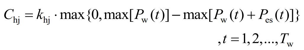
In the formula, Khj is the unit cost of the delayed passage. In order to avoid overcharging and discharging during the process of composite energy storage to suppress wind power fluctuations, and to have sufficient charging and discharging response capabilities, the following constraints are imposed on the energy storage SOC and charging and discharging power:
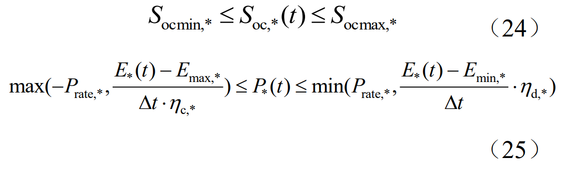
In the formula, Soc, * (t) is the state of charge of energy storage at time t; Emax, *, Emin, * are the upper and lower limits of the energy state, respectively; Δ T is the sampling interval.
3.Model solving process based on IEHHO algorithm
HHO is a gradient free optimization algorithm that simulates the predatory behavior of Harris eagles. The optimization process includes the global search stage, the transition stage from global search to local search, and the local search stage. It has the characteristics of simple principle and strong applicability [23]. Due to the fact that the model in this article is a multimodal complex model, there are shortcomings in convergence speed and accuracy when applying the HHO algorithm for solving. Therefore, improvements are made to the HHO algorithm to improve its performance. Firstly, introduce an elite system to fully utilize the dominant population and increase population diversity to improve the convergence speed and accuracy of the algorithm; Then, a nonlinear energy factor update strategy was designed to balance the global and local search capabilities of the algorithm at each time period, and a Gaussian random walk strategy was introduced to avoid the algorithm falling into local optima. The proposed model solving process based on the IEHHO algorithm is as follows.
Initialize the population with SG filtering parameters, namely window length and polynomial fitting order, as decision variables, and obtain the corresponding net benefit value through a capacity optimization model.
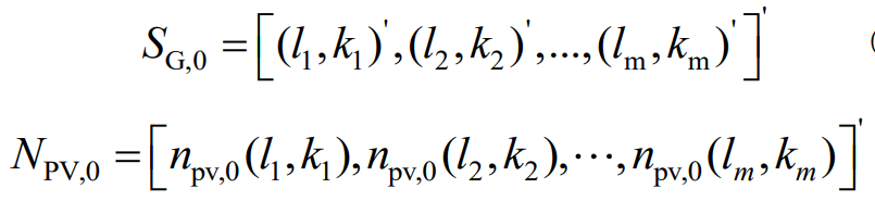
In the formula, SG, 0 is the initial filtering parameter set; NPV, 0 is the set of net present values; Li and ki are the filtering window length and polynomial fitting order corresponding to the i-th individual; NPV (·) is the present value function of net benefits.
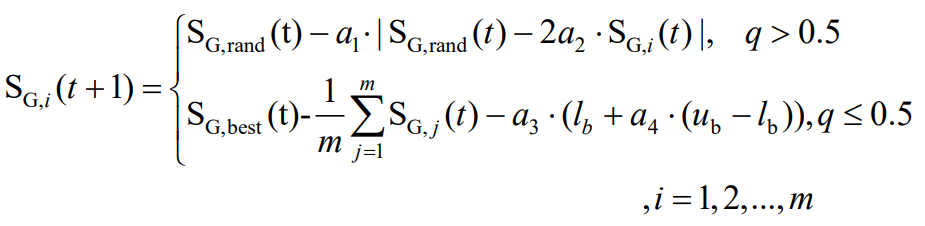
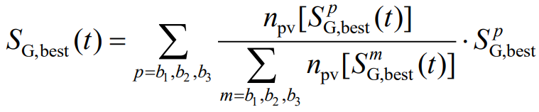
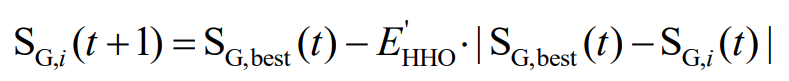
Firstly, a random search is conducted globally, as shown in equation (28). In this process, in order to avoid a decrease in population diversity and falling into local optima during the later optimization process, an elite hierarchy system is introduced to strengthen the information sharing of suboptimal solutions during the iteration process. Taking into account the top three filtering parameter groups with net benefit values as equivalent optimal individuals, as shown in equation (29), other filtering parameter groups are updated.
In the formula, SG, rand are the randomly selected filtering parameter groups in the population; SG, best, SPG, and best are the equivalent optimal filtering parameter group and the filtering parameter group corresponding to the p-th net benefit value in the population, respectively; B is the three sets of filtering parameters with the best net benefit; q. A1, a2, a3, and a4 are random numbers of [0,1]; UB and lb are the upper and lower limits of the filtering parameter group value range.
1) | E’HHO | > 1
Among them,
Secondly, the conversion from global search to local search is controlled by the energy function algorithm. In the HHO algorithm, the process adopts a linear update method, which only performs local search in the second half of the iteration, which is prone to falling into local optima. Therefore, a nonlinear energy function update method is proposed to balance the global search and local search in the later stage.
In the formula, tH is the current number of iterations; TH, max is the maximum number of iterations; Rand is a random number in [0,1].
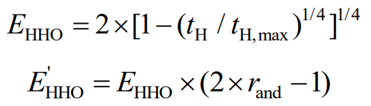
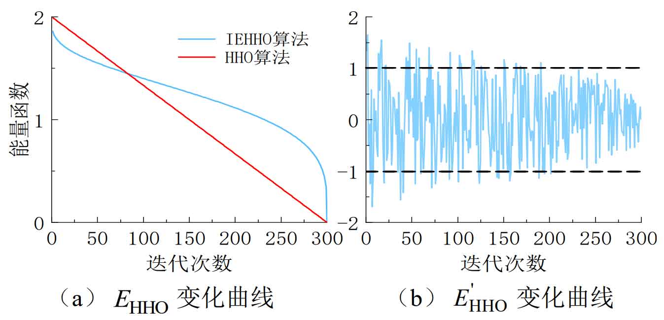
As shown in Figure 1, compared to the HHO linear update strategy, the energy function under the new strategy can control the algorithm’s global search ability in the early iteration stage; Being able to balance global and local search capabilities in the middle of an iteration; In the later stage of the iteration, local search is mainly carried out, while preserving the possibility of global search.
Then select the local search mode based on the energy function E’HHO and the random number r.
2) | E’HHO | ≥ 0.5 and r ≥ 0.5
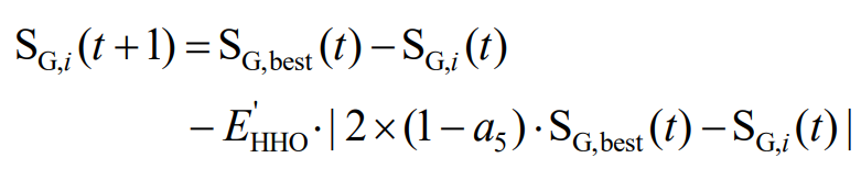
3) | E’HHO | ≥ 0.5 and r<0.5
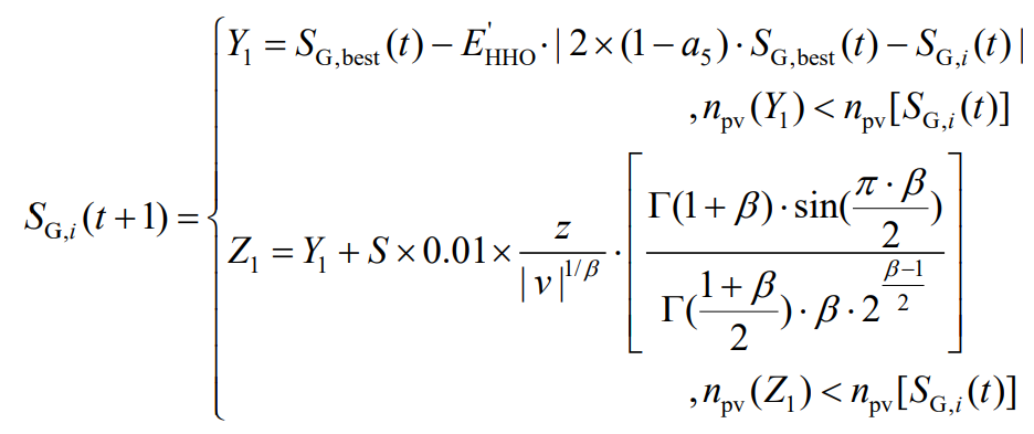
4) | E’HHO |<0.5 and r ≥ 0.5
4) | E’HHO |<0.5 and r < 0.5
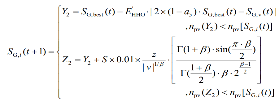
In the formula, r, a5, z, and v are all random numbers of [0,1]; β Is a constant, taken as 1.5; S is a two-dimensional random vector; Γ (·) is a gamma function.
At the same time, to avoid algorithm stagnation, a Gaussian random walk strategy is introduced during the iteration process. If the equivalent filter parameter group SG, best, does not change after m consecutive iterations, the algorithm is considered to be at a standstill. At this point, a new individual is generated through equation (32), which then causes the algorithm to jump out of local optima.
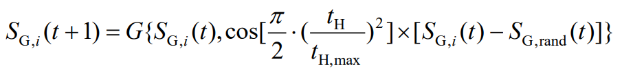
In the equation, G (·) is a Gaussian function.
Considering the SG filtering parameter constraints in the internal power decoupling strategy, l and k are taken as integers during the iteration process, and k<l. Finally, repeat the above process until the maximum number of iterations is reached.
4.Conclusion
This article proposes a composite energy storage capacity configuration method suitable for suppressing wind power fluctuations based on the independent approach of composite energy storage total power allocation and internal power decoupling process. The calculation example shows that:
(1) The proposed adaptive time window wavelet packet method can balance the overall wind power smoothing and local wind power tracking, achieve better composite energy storage total power, and have good adaptability in different power fluctuation scenarios. Compared to wavelet packet decomposition, the proposed method reduces the maximum smoothing power by 29%; The cumulative maximum suppression energy decreased by 43.36%; The total suppressed energy decreased by 73.38%, and the cumulative maximum suppressed energy variation in both scenarios decreased from 44.57% to 13.98%, while the total suppressed energy decreased from 52.19% to 13.10%.
(2) The internal power based on SG filtering decoupling conforms to the composite energy storage output characteristics; The capacity configuration scheme obtained from the full life cycle cost-benefit model can meet the demand for wind power fluctuation suppression while ensuring economic feasibility; The proposed IEHHO algorithm has improved the model solving efficiency, with a 13.1% and 0.72% increase in solving speed and convergence accuracy, respectively.