
The accurate and reliable prediction of the State of Charge (SOC) for lithium-ion batteries is a cornerstone of modern battery management systems (BMS). As the primary energy storage solution for electric vehicles (EVs), portable electronics, and grid storage, understanding the precise remaining capacity of a lithium-ion battery is critical for optimizing performance, ensuring operational safety, preventing overcharge/discharge, and extending the overall service life. SOC, defined as the ratio of remaining capacity to maximum available capacity, serves as a fundamental “fuel gauge.” However, its direct measurement is impractical; it must be estimated from other measurable parameters such as terminal voltage, current, and temperature, which involve complex, non-linear, and time-dependent electrochemical dynamics.
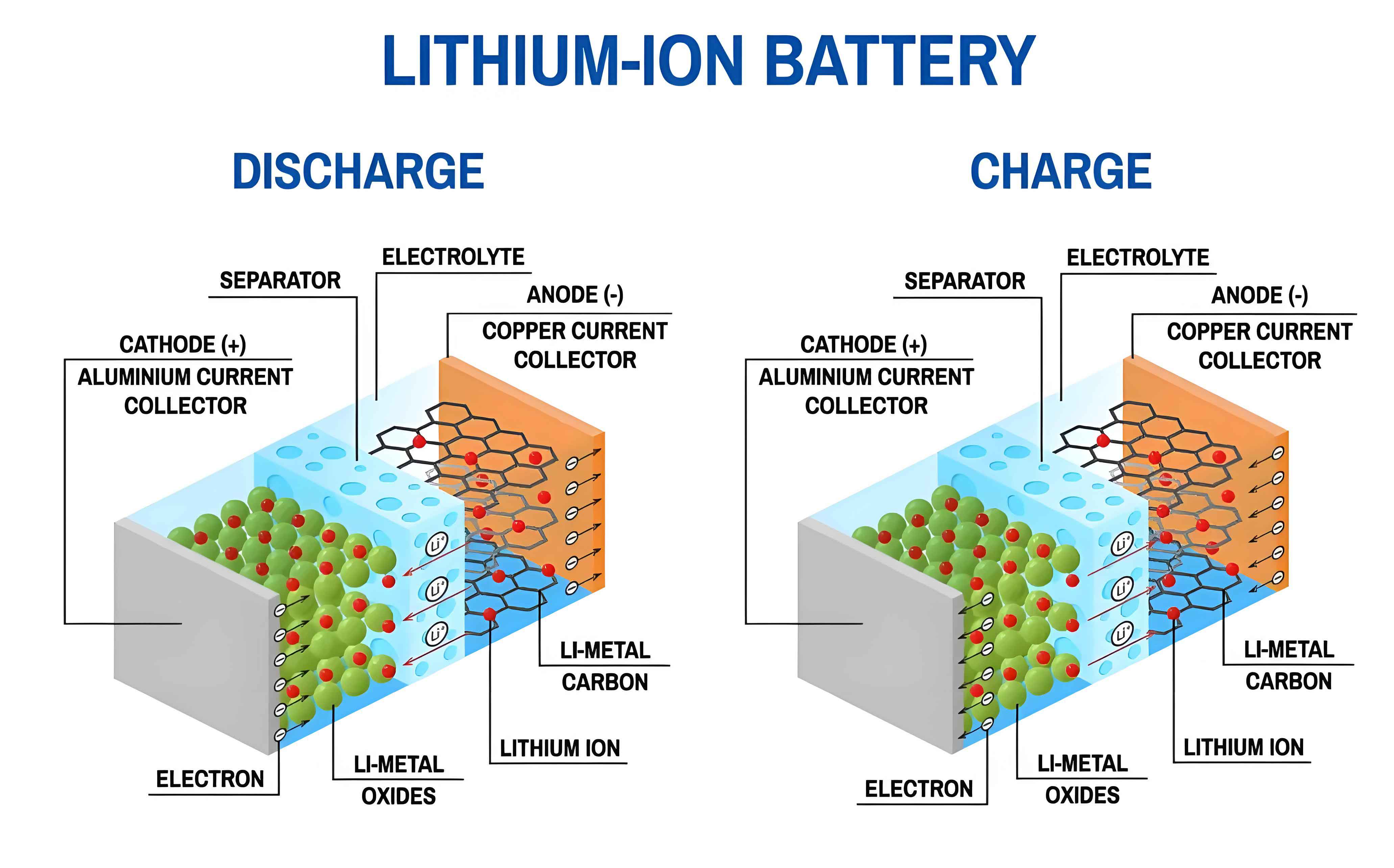
Traditional SOC estimation methodologies can be broadly categorized into model-based and data-driven approaches. Model-based techniques, such as those employing Equivalent Circuit Models (ECMs) combined with state observers like the Kalman Filter (KF) or its variants (EKF, UKF), rely on a priori knowledge of the battery’s physical characteristics. While effective in some scenarios, their accuracy is inherently limited by the fidelity of the underlying model. The intricate internal electrochemistry of a lithium-ion battery is challenging to encapsulate perfectly in a simplified circuit model, leading to estimation errors, especially under dynamic operating conditions and throughout the battery’s aging process.
In recent years, data-driven methods have emerged as powerful alternatives, bypassing the need for explicit physical modeling. By learning complex patterns and non-linear mappings directly from historical operational data, techniques like Artificial Neural Networks (ANNs), Support Vector Machines (SVMs), and notably, Recurrent Neural Networks (RNNs) including Long Short-Term Memory (LSTM) and Gated Recurrent Unit (GRU) networks, have demonstrated remarkable success in SOC prediction. These models inherently capture temporal dependencies in time-series data. However, conventional RNN-based architectures suffer from significant limitations: they process sequences sequentially, which constrains computational speed and parallelization, and they often struggle with capturing very long-range dependencies due to issues like vanishing gradients.
The Transformer architecture, introduced initially for natural language processing, presents a paradigm shift for sequence modeling. Its core mechanism, the self-attention mechanism, allows the model to weigh the importance of all elements in a sequence simultaneously when processing any single element. This property offers two major advantages for time-series prediction: it effectively captures long-term dependencies regardless of distance in the sequence, and it enables highly efficient parallel computation during training. Nevertheless, the standard Transformer encoder is designed to model relationships between elements within a single sequence and may not optimally extract localized, hierarchical features from multi-variate time-series data like battery sensor readings.
To harness the strengths of both deep feature extraction and powerful sequence modeling, we propose a novel hybrid architecture for SOC estimation. Our model synergistically combines a one-dimensional Convolutional Neural Network (CNN) with a Transformer encoder. The CNN front-end acts as a sophisticated feature extractor, processing the raw multi-variate input streams (voltage, current, temperature) to generate a higher-level, condensed feature sequence that encapsulates localized temporal patterns. This refined sequence is then fed into the Transformer encoder. The encoder’s multi-head self-attention mechanism builds a comprehensive global understanding of the entire feature sequence context, learning the complex, long-term dependencies that govern SOC evolution. Finally, a regression head outputs the predicted SOC value. This CNN-Transformer fusion is designed to be more accurate, robust, and computationally efficient than traditional RNN-based approaches for predicting the state of a lithium-ion battery.
The remainder of this article is organized as follows. We first provide a detailed exposition of the proposed methodology, breaking down the mathematical formulations of the CNN and Transformer components. Subsequently, we describe the experimental setup, including the battery datasets used and the implementation details of our model. We then present and discuss the results, showcasing the performance of our model under various dynamic driving cycles and temperature conditions, and include a comparative analysis against other state-of-the-art data-driven models. Finally, we conclude with a summary of our contributions and potential directions for future work.
Methodology: The CNN-Transformer Hybrid Architecture
The core objective of our model is to learn a mapping function \( f \) from a sequence of historical battery measurements to the current SOC value. Let the input at time \( t \) be a vector \( \mathbf{x}_t = [V_t, I_t, T_t] \), where \( V_t \) is terminal voltage, \( I_t \) is current (positive for discharge), and \( T_t \) is temperature. Given a look-back window of length \( L \), the input to the model is a matrix \( \mathbf{X} = [\mathbf{x}_{t-L+1}, \mathbf{x}_{t-L+2}, …, \mathbf{x}_{t}]^T \in \mathbb{R}^{L \times 3} \). The model outputs the predicted SOC at time \( t \), denoted as \( \widehat{SOC}_t \).
The architecture, as illustrated in the conceptual diagram, consists of three primary stages: 1) Convolutional Feature Extraction, 2) Context Encoding with Transformer, and 3) Regression Output.
1. Convolutional Feature Extraction
The one-dimensional CNN processes the input sequence \( \mathbf{X} \) to extract salient local temporal features. A 1D convolutional layer applies a set of learnable filters (kernels) that slide along the temporal dimension. For a single filter with kernel size \( k_s \) and weights \( \mathbf{W}^{(c)} \in \mathbb{R}^{k_s \times d_{in}} \), where \( d_{in}=3 \), the operation at position \( i \) in the sequence produces a feature \( c_i \):
$$
c_i = \sigma\left( \sum_{m=0}^{k_s-1} \sum_{n=1}^{d_{in}} \mathbf{W}^{(c)}_{m, n} \cdot \mathbf{X}_{i+m, n} + b^{(c)} \right)
$$
where \( \sigma \) is a non-linear activation function (e.g., ReLU), and \( b^{(c)} \) is the bias term. By employing multiple filters (\( N_f \)), the layer generates a new feature map \( \mathbf{C} \in \mathbb{R}^{(L-k_s+1) \times N_f} \). We typically use two consecutive 1D convolutional layers, often interleaved with pooling layers (e.g., MaxPooling) to reduce sequence length and computational complexity while promoting translational invariance. The output of the CNN block is a refined feature matrix \( \mathbf{H}_{cnn} \in \mathbb{R}^{L’ \times d_{model}} \), where \( L’ \) is the reduced sequence length and \( d_{model} \) is the chosen feature dimension for the Transformer.
2. Context Encoding with Transformer
The sequence \( \mathbf{H}_{cnn} \) is then passed to a Transformer encoder. The encoder is composed of a stack of \( N \) identical layers, each containing two sub-layers: a Multi-Head Self-Attention (MHSA) mechanism and a position-wise Feed-Forward Network (FFN).
a) Multi-Head Self-Attention: This is the core mechanism that establishes relationships across all time steps. For the input sequence \( \mathbf{H} \in \mathbb{R}^{L’ \times d_{model}} \), linear projections are used to create Query (\( \mathbf{Q} \)), Key (\( \mathbf{K} \)), and Value (\( \mathbf{V} \)) matrices:
$$ \mathbf{Q} = \mathbf{H}\mathbf{W}^Q, \quad \mathbf{K} = \mathbf{H}\mathbf{W}^K, \quad \mathbf{V} = \mathbf{H}\mathbf{W}^V $$
where \( \mathbf{W}^Q, \mathbf{W}^K, \mathbf{W}^V \in \mathbb{R}^{d_{model} \times d_k} \). The scaled dot-product attention for a single head is computed as:
$$ \text{Attention}(\mathbf{Q}, \mathbf{K}, \mathbf{V}) = \text{softmax}\left(\frac{\mathbf{Q}\mathbf{K}^T}{\sqrt{d_k}}\right)\mathbf{V} $$
The scaling factor \( \sqrt{d_k} \) prevents vanishing gradients. Multi-head attention runs \( h \) such attention operations in parallel (with different linear projection weights), concatenates the results, and projects them back:
$$ \text{MultiHead}(\mathbf{H}) = \text{Concat}(\text{head}_1, …, \text{head}_h) \mathbf{W}^O $$
$$ \text{where head}_i = \text{Attention}(\mathbf{H}\mathbf{W}_i^Q, \mathbf{H}\mathbf{W}_i^K, \mathbf{H}\mathbf{W}_i^V) $$
This allows the model to jointly attend to information from different representation subspaces at different positions, which is crucial for understanding the multi-faceted dependencies in lithium-ion battery data.
b) Position-wise Feed-Forward Network: After attention, each position’s representation is independently transformed by a simple FFN, typically consisting of two linear transformations with a ReLU activation in between:
$$ \text{FFN}(x) = \max(0, x\mathbf{W}_1 + b_1)\mathbf{W}_2 + b_2 $$
Each sub-layer is followed by a residual connection and layer normalization. This structure enables stable and deep network training.
Since the Transformer lacks inherent notion of sequence order, positional encodings \( \mathbf{P} \in \mathbb{R}^{L’ \times d_{model}} \) are added to the input features: \( \mathbf{H}_{input} = \mathbf{H}_{cnn} + \mathbf{P} \). The output of the encoder stack is a context-rich representation \( \mathbf{Z} \in \mathbb{R}^{L’ \times d_{model}} \).
3. Regression Output
To produce the final SOC prediction, we aggregate the information across the temporal dimension. A common approach is to use global average pooling on the encoder output sequence \( \mathbf{Z} \), resulting in a single vector \( \mathbf{z}_{pooled} \in \mathbb{R}^{d_{model}} \) that summarizes the entire context window. This vector is then passed through one or more fully connected (dense) layers to perform the regression:
$$
\widehat{SOC}_t = \mathbf{W}_{out} \cdot \text{ReLU}(\mathbf{W}_{fc} \cdot \mathbf{z}_{pooled} + \mathbf{b}_{fc}) + b_{out}
$$
The entire model—CNN filters, Transformer weights, and regression layers—is trained end-to-end by minimizing the mean squared error (MSE) between the predicted and true SOC values over the training dataset using backpropagation and an optimizer like Adam.
| Method Category | Key Principle | Advantages | Disadvantages |
|---|---|---|---|
| Model-Based (e.g., KF with ECM) | Uses a mathematical battery model and a recursive filter for state estimation. | Provides uncertainty bounds. Works well with accurate models. | Model inaccuracy leads to error. Sensitive to noise statistics. Computationally complex for high-fidelity models. |
| Data-Driven – RNN/LSTM | Learns temporal dynamics directly from data using recurrent neural units. | Excellent at capturing sequential patterns. High accuracy with sufficient data. | Sequential processing limits training speed (hard to parallelize). Potential issues with very long-term dependencies. |
| Data-Driven – Standard Transformer | Uses self-attention to model all pairwise dependencies in a sequence. | Superior long-range dependency capture. Highly parallelizable training. | May require large datasets. Can be computationally intensive for very long sequences. Less focus on local feature extraction. |
| Proposed CNN-Transformer | Combines local feature extraction (CNN) with global context modeling (Transformer). | Excels at both local pattern and long-term dependency capture. Parallelizable and efficient. Robust to dynamic conditions. | More complex than simple models. Requires careful hyperparameter tuning. |
Experimental Setup and Data Preparation
To validate the effectiveness of our proposed hybrid model for lithium-ion battery SOC prediction, we conducted extensive experiments using publicly available battery aging datasets.
Dataset: We utilized data from the extensive battery testing carried out by the Center for Advanced Life Cycle Engineering (CALCE) at the University of Maryland. The data pertains to commercial 18650-type lithium iron phosphate (LFP) cells. Crucially, the tests cover multiple dynamic driving profiles that closely mimic real-world EV operation, including:
- Dynamic Stress Test (DST): A simplified but aggressive profile with step changes in current.
- Federal Urban Driving Schedule (FUDS): Represents stop-and-go city driving conditions.
- US06 Highway Driving Schedule: Represents high-speed, aggressive highway driving.
Tests were performed at various controlled ambient temperatures (e.g., 0°C, 25°C, 45°C), which is vital as the performance and dynamics of a lithium-ion battery are highly temperature-dependent. For each cycle, measurements of voltage (V), current (A), and calculated SOC (via Coulomb counting with careful calibration) were recorded.
Data Preprocessing: The raw time-series data was segmented into sequences using a sliding window approach. For a given time step \( t \), the input features were the past \( L \) measurements of \( [V, I, T] \), and the target label was the SOC at time \( t \). The data was normalized to have zero mean and unit variance per feature across the training set to stabilize and accelerate the training process. We structured our experiment to test generalizability: models were trained on data from DST and US06 cycles at multiple temperatures and then evaluated on the completely unseen FUDS cycle at those same temperatures.
Model Implementation & Hyperparameters: The model was implemented using the PyTorch deep learning framework. After empirical tuning, the key hyperparameters were set as follows. The CNN module consisted of two 1D convolutional layers with 64 filters each, kernel size of 3, ReLU activation, and followed by a MaxPool1d layer. The Transformer encoder had \( N=3 \) layers, with \( d_{model}=32 \), \( h=2 \) attention heads, and a feed-forward dimension of 128. The look-back window length \( L \) was set to 50 time steps. The model was trained using the Adam optimizer with a learning rate of 0.001, a batch size of 64, and for 10 epochs. The loss function was Mean Squared Error (MSE).
| Parameter | Specification / Value |
|---|---|
| Battery Type | 18650 Lithium Iron Phosphate (LFP) |
| Source | University of Maryland CALCE Group |
| Driving Cycles | DST, FUDS, US06 |
| Temperatures | 0°C, 25°C, 45°C |
| Training Data | DST + US06 cycles |
| Testing Data | FUDS cycle (unseen during training) |
| Input Features (per time step) | Voltage (V), Current (A), Temperature (°C) |
| Target Variable | State of Charge (SOC) [0-1] |
| Look-back Window (L) | 50 |
Results and Discussion
We evaluated the performance of our CNN-Transformer model using standard regression metrics: Mean Absolute Error (MAE), Root Mean Squared Error (RMSE), and Mean Absolute Percentage Error (MAPE). The formulas are given below, where \( n \) is the number of samples, \( y_i \) is the true SOC, and \( \hat{y}_i \) is the predicted SOC.
$$
\begin{aligned}
\text{MAE} &= \frac{1}{n} \sum_{i=1}^{n} |y_i – \hat{y}_i| \\
\text{RMSE} &= \sqrt{\frac{1}{n} \sum_{i=1}^{n} (y_i – \hat{y}_i)^2} \\
\text{MAPE} &= \frac{100\%}{n} \sum_{i=1}^{n} \left| \frac{y_i – \hat{y}_i}{y_i} \right|
\end{aligned}
$$
Performance Across Temperatures: The primary results for the proposed model on the test set (FUDS cycle) at three different temperatures are summarized in Table 3. The model demonstrates consistently high accuracy and robustness. At the nominal 25°C condition, the model achieves an outstanding MAE of 0.41% and an RMSE of 0.93%. More importantly, it maintains excellent performance under the challenging low-temperature (0°C) and high-temperature (45°C) conditions, with average MAEs of 0.78% and 0.53%, respectively. The overall average MAE across temperatures is 0.57%. This indicates that the CNN-Transformer architecture has successfully learned the underlying electrochemical behavior of the lithium-ion battery that governs SOC, and this learning generalizes well across different thermal environments. The small MAPE values further confirm the high estimation precision throughout the entire discharge range.
| Test Condition | MAE (%) | RMSE (%) | MAPE (%) |
|---|---|---|---|
| FUDS at 0°C | 0.78 | 1.17 | 1.61 |
| FUDS at 25°C | 0.41 | 0.93 | 1.08 |
| FUDS at 45°C | 0.53 | 1.02 | 1.05 |
| Average | 0.57 | 1.04 | 1.25 |
The prediction curves for the FUDS cycle at 25°C show an almost perfect overlap between the estimated SOC and the ground truth reference. The error plot reveals that the estimation error is tightly bounded within a ±2% band for the vast majority of the cycle, with no observable error drift or accumulation over time. This performance on a dynamic, realistic driving profile confirms the model’s capability to handle the non-linear and transient behavior of a lithium-ion battery.
Comparative Analysis
To firmly establish the superiority of the proposed approach, we compared it against three other prominent data-driven models using the same 25°C dataset and identical train-test split. The baselines were:
- Gated Recurrent Unit (GRU): A streamlined RNN variant with gating mechanisms.
- CNN-LSTM: A hybrid model using a CNN for feature extraction followed by an LSTM for temporal modeling (a common architecture in recent literature).
- Bidirectional LSTM (BiLSTM): An LSTM that processes sequences both forward and backward, theoretically capturing richer contextual information.
All comparative models were implemented and tuned to their best performance on the same task.
The quantitative results are presented in Table 4. Our CNN-Transformer model significantly outperforms all three baselines across all error metrics. It reduces the MAE by approximately 86% compared to the GRU, 66% compared to the CNN-LSTM, and 46% compared to the BiLSTM. The RMSE and MAPE follow similar trends. This substantial improvement underscores the effectiveness of the Transformer’s self-attention mechanism over recurrent units for modeling the long-term, complex dependencies in lithium-ion battery data. While the CNN-LSTM model also uses a CNN front-end, the LSTM’s sequential processing and potential difficulty with very long-range context appear to be limiting factors that the Transformer overcomes.
| Model | MAE (%) | RMSE (%) | MAPE (%) |
|---|---|---|---|
| GRU | 4.17 | 3.02 | 3.24 |
| CNN-LSTM | 1.66 | 1.86 | 1.71 |
| BiLSTM | 1.05 | 1.13 | 1.21 |
| Proposed CNN-Transformer | 0.41 | 0.93 | 1.08 |
Qualitatively, the prediction curves from the baseline models show greater deviation from the reference, with noticeable oscillations and lag, especially during rapid current transients characteristic of the FUDS cycle. In contrast, the CNN-Transformer prediction is smooth and closely tracks the reference even during these difficult segments. Furthermore, from a computational perspective, the Transformer-based architecture, due to its parallelizability, trained faster per epoch than the sequential BiLSTM and CNN-LSTM models on equivalent hardware, offering a practical advantage for development and deployment.
Conclusion and Future Work
In this work, we have introduced and validated a novel hybrid deep learning architecture for the accurate estimation of the State of Charge in lithium-ion batteries. By integrating a one-dimensional Convolutional Neural Network with a Transformer encoder, the model capitalizes on the complementary strengths of both components: the CNN excels at extracting hierarchical local features from the raw multi-variate time-series data (voltage, current, temperature), while the Transformer’s multi-head self-attention mechanism builds a powerful global context model, capturing complex long-term temporal dependencies critical for SOC dynamics. This synergy allows the model to learn the intricate non-linear mapping from operational measurements to SOC without requiring an explicit electrochemical model.
Experimental results on comprehensive, real-world dynamic driving cycle data (DST, US06, FUDS) across a range of temperatures (0°C, 25°C, 45°C) demonstrate the exceptional performance and robustness of the proposed method. The model achieved an average MAE of only 0.57% on unseen test data, significantly outperforming established baseline models like GRU, CNN-LSTM, and BiLSTM. Its ability to maintain high accuracy under varying thermal conditions confirms its strong generalization capability, which is essential for real-world BMS applications where operating environments are not constant.
The implications of this research are significant for advancing BMS technology. A more accurate and reliable SOC estimate enables optimal charging strategies, improves range prediction for EVs, enhances safety protocols, and contributes to prolonging the lifespan of the lithium-ion battery pack. The parallelizable nature of the Transformer also points towards potential for efficient embedded implementation.
Future work will focus on several promising directions. First, we plan to extend the model to perform joint estimation of SOC and State of Health (SOH), as these states are deeply interrelated. Second, incorporating attention-based decoder structures or sequence-to-sequence frameworks could enable multi-step ahead SOC forecasting, providing predictive capabilities for energy management. Third, exploring knowledge distillation or model compression techniques will be crucial for deploying this accurate but somewhat complex model on resource-constrained edge devices within a BMS. Finally, testing the architecture on a wider variety of lithium-ion battery chemistries (e.g., NMC, LCO) and under more diverse aging conditions will further validate its universality and practical utility.