
In the contemporary power market, characterized by the rapid electrification of transportation and the integration of renewable energy sources, the lithium-ion battery has emerged as the dominant energy storage technology. Its superior energy density, lightweight design, and extended cycle life have positioned it as the core component of modern electric vehicles (EVs) and portable electronics. The safe and reliable operation of these systems is paramount and is intrinsically linked to the degradation state of the lithium-ion battery. A critical metric for quantifying this degradation is the State of Health (SOH), which represents the battery’s current capacity relative to its nominal capacity when new. Accurate SOH estimation is not merely a diagnostic tool; it is fundamental for effective Battery Management Systems (BMS), enabling optimal charging strategies, preventing over-discharge, predicting end-of-life, and ensuring operational safety. This paper details a first-person perspective investigation into developing a data-driven SOH estimation model, leveraging the capabilities of Long Short-Term Memory (LSTM) recurrent neural networks, which are particularly suited for processing the sequential nature of battery cycling data.
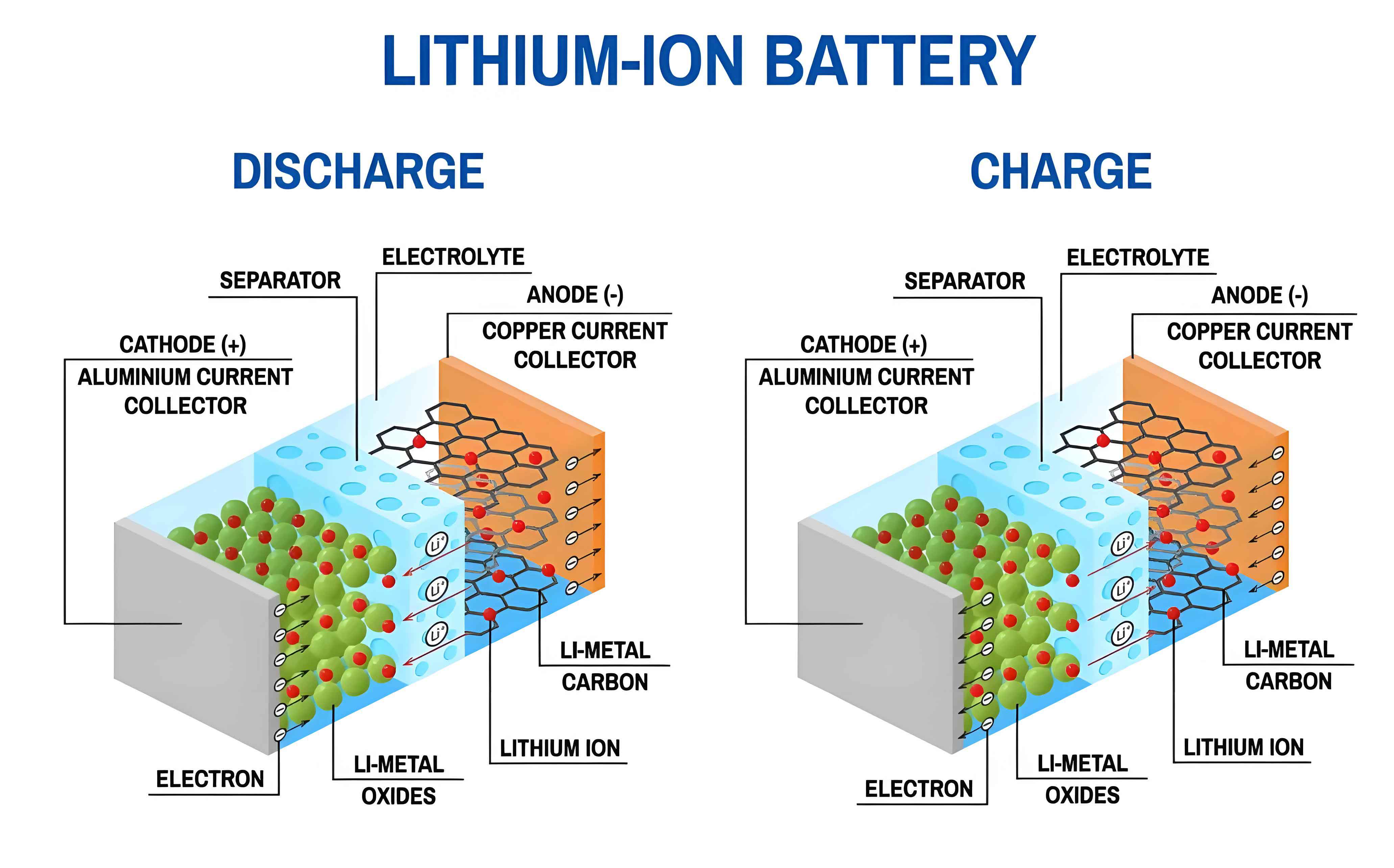
Traditional methods for lithium-ion battery SOH assessment encompass several categories. Direct measurement methods, such as full-capacity tests, offer high accuracy but are impractical for online, in-situ estimation as they require interrupting normal operation. Model-based approaches, including equivalent circuit models or electrochemical models, rely on a deep understanding of internal physicochemical processes, which are complex, non-linear, and challenging to parameterize accurately over a battery’s lifetime. In contrast, data-driven methods bypass the need for explicit physical modeling. Instead, they learn the complex, non-linear relationship between easily measurable operational parameters and the battery’s SOH directly from historical data. Among machine learning techniques, deep learning models like LSTM networks have shown exceptional promise for time-series forecasting, making them ideal for analyzing the temporal evolution of a lithium-ion battery‘s aging characteristics.
1. Feature Selection and Correlation Analysis
The foundation of an effective data-driven model lies in the selection of informative input features. For this study, we utilized the publicly available battery aging dataset from the Center for Advanced Life Cycle Engineering (CALCE). From the operational data of each charge-discharge cycle, we engineered three indicative features that are known to evolve with lithium-ion battery degradation:
1. Constant Current Charging Time (CCCT): The duration of the constant-current phase in a charging protocol. As the lithium-ion battery ages and its internal resistance increases, the time to reach the cutoff voltage typically decreases.
2. Constant Voltage Charging Time (CVCT): The duration of the constant-voltage (taper) charging phase. This time generally increases with aging because a degraded battery requires more time to “top up” its capacity under a constant voltage.
3. Average Discharge Voltage (ADV): The mean voltage during a discharge cycle. This voltage tends to drop as the battery’s usable capacity and overall health diminish.
To quantitatively justify the selection of these features, we performed a Spearman rank correlation analysis. Unlike Pearson correlation, Spearman’s method assesses monotonic relationships, making it robust to non-linearities. The correlation coefficient $$r_s$$ between a feature vector $$X$$ and the SOH vector $$Y$$ is calculated as follows, where $$d_j$$ is the difference between the ranks of corresponding values from $$X$$ and $$Y$$, and $$n$$ is the number of observations:
$$
r_s = 1 – \frac{6 \sum_{j=1}^{n} d_j^2}{n(n^2 – 1)}
$$
The calculated Spearman correlation coefficients for three different cells (CS2-35, CS2-36, CS2-37) are summarized in Table 1. The absolute values of the coefficients are consistently high (>0.86), confirming a strong monotonic relationship. CCCT shows a very strong positive correlation with SOH, while CVCT shows a strong negative correlation. ADV exhibits a strong positive correlation. These results validate that CCCT, CVCT, and ADV are highly relevant features for estimating the SOH of a lithium-ion battery.
| Cell ID | CCCT | CVCT | ADV |
|---|---|---|---|
| CS2-35 | 0.9920 | -0.9390 | 0.9423 |
| CS2-36 | 0.9933 | -0.8675 | 0.9641 |
| CS2-37 | 0.9836 | -0.9370 | 0.9558 |
2. LSTM Neural Network Model Architecture
Recurrent Neural Networks (RNNs) are designed for sequential data. However, standard RNNs suffer from the vanishing gradient problem, making it difficult to learn long-term dependencies. The Long Short-Term Memory (LSTM) network overcomes this limitation through a gated cell structure. The core of the LSTM cell is the cell state $$C_t$$, which acts as a conveyor belt of information, regulated by three gates:
- Forget Gate ($$f_t$$): Decides what information to discard from the cell state. It looks at the previous hidden state $$h_{t-1}$$ and the current input $$x_t$$.
- Input Gate ($$i_t$$): Decides what new information to store in the cell state. It has two parts: a sigmoid layer that decides which values to update, and a tanh layer that creates a vector of new candidate values, $$\tilde{C}_t$$.
- Output Gate ($$o_t$$): Decides what part of the cell state to output as the hidden state $$h_t$$.
The mathematical formulation of an LSTM cell is as follows:
Forget Gate:
$$ f_t = \sigma(W_f \cdot [h_{t-1}, x_t] + b_f) $$
Input Gate and Candidate Value:
$$ i_t = \sigma(W_i \cdot [h_{t-1}, x_t] + b_i) $$
$$ \tilde{C}_t = \tanh(W_C \cdot [h_{t-1}, x_t] + b_C) $$
Cell State Update:
$$ C_t = f_t * C_{t-1} + i_t * \tilde{C}_t $$
Output Gate and Hidden State:
$$ o_t = \sigma(W_o \cdot [h_{t-1}, x_t] + b_o) $$
$$ h_t = o_t * \tanh(C_t) $$
Here, $$W$$ and $$b$$ represent weight matrices and bias vectors, respectively, $$\sigma$$ denotes the sigmoid activation function, and $$*$$ represents element-wise multiplication. This gated mechanism allows the LSTM to selectively remember or forget information over long sequences, making it exceptionally capable of modeling the long-term trends in lithium-ion battery capacity fade.
The network architecture for our SOH estimation model consisted of an input layer, two LSTM hidden layers (with 64 and 32 units, respectively), and a fully connected output layer to produce the SOH estimate. To train the network, we used the Adam (Adaptive Moment Estimation) optimizer, which combines the advantages of two other extensions of stochastic gradient descent: AdaGrad and RMSProp. The Adam update rules for a parameter $$w$$ at time step $$t$$ are:
Compute biased first and second moment estimates:
$$ m_t = \beta_1 m_{t-1} + (1 – \beta_1) g_t $$
$$ v_t = \beta_2 v_{t-1} + (1 – \beta_2) g_t^2 $$
Compute bias-corrected estimates:
$$ \hat{m}_t = \frac{m_t}{1 – \beta_1^t} $$
$$ \hat{v}_t = \frac{v_t}{1 – \beta_2^t} $$
Update parameters:
$$ w_t = w_{t-1} – \frac{\eta}{\sqrt{\hat{v}_t} + \epsilon} \hat{m}_t $$
where $$g_t$$ is the gradient, $$\eta$$ is the learning rate, $$\beta_1$$ and $$\beta_2$$ are decay rates (typically 0.9 and 0.999), and $$\epsilon$$ is a small constant for numerical stability. Adam’s adaptive learning rates for each parameter make it well-suited for training deep networks efficiently.
3. Experimental Procedure and Hyperparameter Tuning
We applied the proposed methodology to three distinct lithium-ion battery cells from the CALCE dataset: CS2_35, CS2_36, and CS2_37. For each cell, the first 600 charge-discharge cycles were extracted. The feature vectors (CCCT, CVCT, ADV) for these cycles were normalized and used as the input sequence. The corresponding SOH values (calculated as the ratio of current maximum available capacity to initial capacity) served as the target labels. The dataset for each cell was split 1:1 into a training set (cycles 1-300) and a testing set (cycles 301-600).
A critical aspect of deep learning is hyperparameter optimization. We employed a trial-and-error (grid search) approach to find a robust configuration. The number of neurons in the two LSTM layers was fixed at 64 and 32, based on preliminary experiments. We then systematically varied two key hyperparameters: the learning rate ($$\eta$$) and the number of training epochs (iterations). The goal was to identify the combination that yielded the most accurate and stable predictions on the unseen test data. Model performance was evaluated using four standard regression metrics:
- Mean Absolute Error (MAE): $$ \text{MAE} = \frac{1}{n} \sum_{i=1}^{n} |y_i – \hat{y}_i| $$
- Root Mean Square Error (RMSE): $$ \text{RMSE} = \sqrt{\frac{1}{n} \sum_{i=1}^{n} (y_i – \hat{y}_i)^2} $$
- Mean Absolute Percentage Error (MAPE): $$ \text{MAPE} = \frac{100\%}{n} \sum_{i=1}^{n} \left| \frac{y_i – \hat{y}_i}{y_i} \right| $$
- Coefficient of Determination (R²): $$ R^2 = 1 – \frac{\sum_{i=1}^{n} (y_i – \hat{y}_i)^2}{\sum_{i=1}^{n} (y_i – \bar{y})^2} $$
Lower values of MAE, RMSE, and MAPE indicate better accuracy, while an R² value closer to 1.0 indicates a better fit.
4. Results, Analysis, and Discussion
The results for each lithium-ion battery cell are presented and analyzed below. The tables compare the evaluation metrics under different hyperparameter settings, and the text describes the corresponding prediction plots.
4.1 Results for Cell CS2_35
Table 2 summarizes the performance metrics for cell CS2_35 under various learning rates and epoch settings. The best performance was achieved with a learning rate of 0.0015 and 200 epochs. This configuration resulted in the lowest MAPE (1.0523%), RMSE (0.0111), and MAE (0.0085), along with the highest R² score (0.8954). Compared to the model trained with a learning rate of 0.001 for 300 epochs, this represents an improvement of approximately 7.4% in MAPE, 7.5% in RMSE, and 7.6% in MAE. The prediction curve for this optimal model closely followed the true SOH degradation trajectory. The LSTM model successfully captured the non-linear capacity fade, with prediction errors remaining consistently low throughout the 300 test cycles. The model’s ability to track the slight curvature in the degradation path demonstrates its effectiveness in learning the long-term temporal dependencies inherent in lithium-ion battery aging data.
| Learning Rate | Epochs | MAPE (%) | RMSE | MAE | R² |
|---|---|---|---|---|---|
| 0.001 | 100 | 1.1134 | 0.0118 | 0.0090 | 0.8808 |
| 0.001 | 200 | 1.0849 | 0.0114 | 0.0088 | 0.8889 |
| 0.001 | 300 | 1.1360 | 0.0120 | 0.0092 | 0.8779 |
| 0.0015 | 200 | 1.0523 | 0.0111 | 0.0085 | 0.8954 |
| 0.002 | 200 | 1.0897 | 0.0115 | 0.0088 | 0.8876 |
4.2 Results for Cell CS2_36
The results for cell CS2_36 are shown in Table 3. For this lithium-ion battery, the optimal configuration was found to be a learning rate of 0.001 trained for 200 epochs. This model achieved a MAPE of 1.1693%, an RMSE of 0.0128, an MAE of 0.0092, and an R² of 0.9428. This performance is superior to training for 300 epochs with the same learning rate, which showed increases in error metrics (MAPE increased by ~16.3%). The prediction plot for the optimal model demonstrates excellent agreement with the actual SOH values. The model accurately predicts the steeper initial fade and the subsequent gradual decline, with the prediction line almost indistinguishable from the true values for a significant portion of the test cycles. The high R² value of 0.94 indicates that the model explains 94% of the variance in the SOH data, highlighting the strong predictive capability of the LSTM network for this cell.
| Learning Rate | Epochs | MAPE (%) | RMSE | MAE | R² |
|---|---|---|---|---|---|
| 0.001 | 100 | 1.0719 | 0.0147 | 0.0085 | 0.9240 |
| 0.001 | 200 | 1.1693 | 0.0128 | 0.0092 | 0.9428 |
| 0.001 | 300 | 1.3962 | 0.0147 | 0.0109 | 0.9244 |
| 0.0015 | 200 | 1.2080 | 0.0130 | 0.0095 | 0.9413 |
| 0.002 | 200 | 1.2774 | 0.0136 | 0.0100 | 0.9350 |
4.3 Results for Cell CS2_37
Table 4 presents the results for cell CS2_37. This lithium-ion battery exhibited the best overall estimation accuracy among the three. The optimal model, trained with a learning rate of 0.001 for 200 epochs, achieved remarkable metrics: a MAPE of only 0.5665%, an RMSE of 0.0061, an MAE of 0.0047, and an R² of 0.9263. This represents a model accuracy of approximately 99.43% (100% – MAPE). The improvement over the 300-epoch model is significant, with a reduction in MAPE of about 15.4%. The corresponding prediction plot shows an almost perfect overlay of the predicted and true SOH curves. The error is minimal and uniform across the entire testing range, showcasing the LSTM model’s exceptional ability to generalize the aging pattern for this particular cell. The consistency of low error across all three cells, despite their individual aging characteristics, strongly validates the robustness of the chosen features (CCCT, CVCT, ADV) and the LSTM architecture for lithium-ion battery SOH estimation.
| Learning Rate | Epochs | MAPE (%) | RMSE | MAE | R² |
|---|---|---|---|---|---|
| 0.001 | 100 | 0.6577 | 0.0074 | 0.0054 | 0.8919 |
| 0.001 | 200 | 0.5665 | 0.0061 | 0.0047 | 0.9263 |
| 0.001 | 300 | 0.6698 | 0.0074 | 0.0055 | 0.8936 |
| 0.0015 | 200 | 0.5710 | 0.0062 | 0.0047 | 0.9244 |
| 0.002 | 200 | 0.5834 | 0.0064 | 0.0048 | 0.9208 |
5. Conclusion
This investigation has demonstrated the high accuracy and feasibility of using Long Short-Term Memory neural networks for the online estimation of lithium-ion battery State of Health. By leveraging easily measurable operational features—constant current charging time, constant voltage charging time, and average discharge voltage—the LSTM model effectively learned the complex, non-linear, and temporal patterns of battery degradation. Through systematic hyperparameter tuning via a trial-and-error approach, optimal model configurations were identified for three different battery cells. The evaluation metrics (MAPE, RMSE, MAE, R²) confirmed that all models achieved high precision, with estimation accuracies exceeding 98%. Notably, the model for cell CS2_37 achieved an accuracy of approximately 99.43%. The results underscore the superiority of the data-driven LSTM approach over more traditional methods, as it requires no explicit knowledge of the internal electrochemical processes of the lithium-ion battery yet delivers highly reliable predictions. Future work will focus on enhancing model generalizability across a wider range of battery types, chemistries, and operational conditions, and on implementing these algorithms for real-time SOH estimation within embedded battery management systems to further improve the safety and longevity of lithium-ion battery packs.