
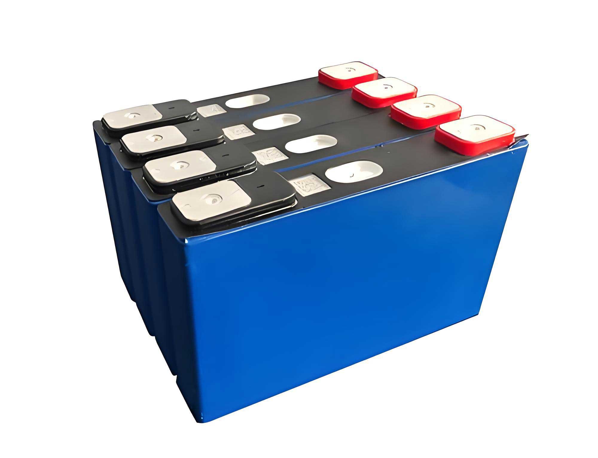
In the realm of new energy vehicles, lithium-ion batteries serve as the core component of the three-electric system. Among various material systems, the LiFePO4 battery stands out due to its high safety, low cost, and long cycle life, making it a favorable choice for both manufacturers and customers. With ongoing optimizations in cell manufacturing and battery pack design, the low-temperature performance and energy density of LiFePO4 batteries have further improved, leading to their increasing adoption in battery electric vehicles (BEVs), plug-in hybrid electric vehicles (PHEVs), and hybrid electric vehicles (HEVs). However, the intrinsic electrochemical properties of LiFePO4 batteries, such as a flat open-circuit voltage (OCV) variation with state of charge (SOC) and significant hysteresis voltage, pose substantial challenges for accurate battery state estimation, including SOC. Therefore, there is a pressing need to develop high-precision battery models to enhance the estimation accuracy for LiFePO4 batteries.
Accurate SOC estimation is a critical function of the battery management system (BMS), as it helps prevent battery abuse like overcharging and over-discharging, thereby improving safety and lifespan. Current SOC estimation methods primarily fall into three categories: (1) ampere-hour integration combined with OCV correction, which is widely used but suffers from errors due to the flat OCV-SOC curve and hysteresis in LiFePO4 batteries; (2) black-box model algorithms, such as artificial neural networks and support vector machines, which offer high accuracy but require substantial computational resources and extensive training data; and (3) Kalman filter-based algorithms using equivalent circuit models, such as extended Kalman filter (EKF), which provide online, closed-loop estimation with good accuracy and error correction capabilities. While equivalent circuit models, like the Rint, Thevenin, and dual-polarization models, are commonly employed, they often neglect the asymmetric hysteresis and polarization characteristics during charging and discharging of LiFePO4 batteries. To address this gap, we propose a novel asymmetric equivalent circuit modeling approach that accounts for these asymmetries, aiming to boost SOC estimation precision for LiFePO4 batteries.
The modeling of LiFePO4 batteries requires careful consideration of their unique electrochemical behaviors. Due to phase transitions during lithium insertion and extraction in active materials, asymmetric hysteresis occurs, which directly influences material properties and must be incorporated into the model. Based on this, we develop an asymmetric equivalent circuit model for LiFePO4 batteries, building upon a second-order RC structure. The model distinguishes between charging and discharging processes by using separate parameters to describe hysteresis and polarization. The circuit schematic includes components such as ohmic resistance (R0), polarization resistances (RD1, RD2), polarization capacitances (CD1, CD2), open-circuit voltage (UOCV), hysteresis voltage (Uh), and terminal voltage (Ut). Subscripts “chr” and “dis” denote charging and discharging, respectively, with current I > 0 for charging and I < 0 for discharging. This asymmetry allows the model to better mimic the real-world behavior of LiFePO4 batteries.
The state of charge (SOC) is defined as the accumulated charge over time, given by the equation:
$$ SOC = SOC_0 + \int \frac{\eta (I – I_{\text{self}})}{C_{\text{Capacity}}} dt $$
where SOC0 is the initial SOC, I is the operating current, Iself is the self-discharge current (negligible for LiFePO4 batteries), η is the Coulombic efficiency, and CCapacity is the rated capacity. Discretizing this yields:
$$ SOC[k] = SOC[k-1] + \frac{\eta I[k] \Delta t}{C_{\text{Capacity}}} $$
The hysteresis voltage Uh is modeled as a function of SOC and time, capturing its dependence on charge-discharge history. The differential equation for hysteresis is:
$$ \frac{dU_h}{dt} =
\begin{cases}
\beta_{\text{chr}} \frac{dSOC}{dt} (U_{h,\text{max}} – U_h) & \text{for charging} \\
\beta_{\text{dis}} \frac{dSOC}{dt} (-U_{h,\text{max}} – U_h) & \text{for discharging}
\end{cases} $$
Here, β represents the hysteresis rate coefficient, which varies with temperature and SOC, and Uh,max is the maximum main hysteresis voltage, calculated as:
$$ U_{h,\text{max}} = \frac{U_{\text{OCV,chr}} – U_{\text{OCV,dis}}}{2} $$
Discretizing the hysteresis equation gives:
$$ U_h[k] =
\begin{cases}
U_h[k-1] + \beta_{\text{chr}} \frac{I_{\text{chr}} \Delta t}{C_{\text{Capacity}}} (U_{h,\text{max}} – U_h[k-1]) & \text{for charging} \\
U_h[k-1] + \beta_{\text{dis}} \frac{I_{\text{dis}} \Delta t}{C_{\text{Capacity}}} (U_{h,\text{max}} + U_h[k-1]) & \text{for discharging}
\end{cases} $$
For polarization dynamics, the state equations for the RC pairs are derived from Kirchhoff’s laws:
$$ \dot{U}_{D1} =
\begin{cases}
-\frac{U_{D1,\text{chr}}}{R_{D1,\text{chr}} C_{D1,\text{chr}}} + \frac{I_{\text{chr}}}{C_{D1,\text{chr}}} & \text{for charging} \\
-\frac{U_{D1,\text{dis}}}{R_{D1,\text{dis}} C_{D1,\text{dis}}} + \frac{I_{\text{dis}}}{C_{D1,\text{dis}}} & \text{for discharging}
\end{cases} $$
$$ \dot{U}_{D2} =
\begin{cases}
-\frac{U_{D2,\text{chr}}}{R_{D2,\text{chr}} C_{D2,\text{chr}}} + \frac{I_{\text{chr}}}{C_{D2,\text{chr}}} & \text{for charging} \\
-\frac{U_{D2,\text{dis}}}{R_{D2,\text{dis}} C_{D2,\text{dis}}} + \frac{I_{\text{dis}}}{C_{D2,\text{dis}}} & \text{for discharging}
\end{cases} $$
Discretizing these leads to:
$$ U_{D1}[k] =
\begin{cases}
U_{D1}[k-1] \times e^{-\frac{\Delta t}{R_{D1,\text{chr}} C_{D1,\text{chr}}}} + \left(1 – e^{-\frac{\Delta t}{R_{D1,\text{chr}} C_{D1,\text{chr}}}}\right) \times I_{\text{chr}}[k] & \text{for charging} \\
U_{D1}[k-1] \times e^{-\frac{\Delta t}{R_{D1,\text{dis}} C_{D1,\text{dis}}}} + \left(1 – e^{-\frac{\Delta t}{R_{D1,\text{dis}} C_{D1,\text{dis}}}}\right) \times I_{\text{dis}}[k] & \text{for discharging}
\end{cases} $$
$$ U_{D2}[k] =
\begin{cases}
U_{D2}[k-1] \times e^{-\frac{\Delta t}{R_{D2,\text{chr}} C_{D2,\text{chr}}}} + \left(1 – e^{-\frac{\Delta t}{R_{D2,\text{chr}} C_{D2,\text{chr}}}}\right) \times I_{\text{chr}}[k] & \text{for charging} \\
U_{D2}[k-1] \times e^{-\frac{\Delta t}{R_{D2,\text{dis}} C_{D2,\text{dis}}}} + \left(1 – e^{-\frac{\Delta t}{R_{D2,\text{dis}} C_{D2,\text{dis}}}}\right) \times I_{\text{dis}}[k] & \text{for discharging}
\end{cases} $$
The output observation equation for terminal voltage is:
$$ U_t[k] = U_{\text{OCV}}[k] + U_0[k] + U_{D1}[k] + U_{D2}[k] $$
where U0[k] = I[k] R0. To estimate SOC, we employ an extended Kalman filter (EKF) algorithm, which recursively minimizes estimation variance. The state-space representation for EKF is:
$$
\begin{aligned}
\mathbf{x}[k] &= \mathbf{F} \mathbf{x}[k-1] + \mathbf{D} u[k] + \omega[k] \\
z[k] &= \mathbf{H} \mathbf{x}[k] + \mathbf{E} u[k] + U_h[k] + \upsilon[k]
\end{aligned}
$$
with state vector \(\mathbf{x} = [SOC, U_{D1}, U_{D2}]^T\), input \(u = I\), and output \(z = U_t\). The matrices are defined as:
$$
\mathbf{F} =
\begin{bmatrix}
1 & 0 & 0 \\
0 & e^{-\frac{\Delta t}{R_{D1}C_{D1}}} & 0 \\
0 & 0 & e^{-\frac{\Delta t}{R_{D2}C_{D2}}}
\end{bmatrix},
\quad
\mathbf{D} =
\begin{bmatrix}
\frac{\eta \Delta t}{C_{\text{Capacity}}} & 0 & 0 \\
0 & 1 – e^{-\frac{\Delta t}{R_{D1}C_{D1}}} & 0 \\
0 & 0 & 1 – e^{-\frac{\Delta t}{R_{D2}C_{D2}}}
\end{bmatrix}
$$
$$
\mathbf{H} = \left[ \frac{dU_{\text{OCV,mid}}}{dSOC}, 1, 1 \right], \quad \mathbf{E} = [R_0]
$$
where UOCV,mid is the average OCV curve. The EKF process involves prediction and correction steps to update SOC estimates based on voltage measurements, ensuring robustness against noise and initial errors.
Parameter identification is crucial for model accuracy. We conduct experiments on a commercial LiFePO4 battery with specifications listed in Table 1, all tests performed at 20°C. The parameters to identify include: (1) OCV curves, (2) hysteresis parameters Uh,max and β, and (3) polarization parameters R0, RD1, CD1, RD2, and CD2 for charging and discharging separately.
| Parameter | Value |
|---|---|
| Rated Capacity | 105 Ah |
| Nominal Voltage | 3.2 V |
| Charge Cut-off Voltage | 3.65 V |
| Discharge Cut-off Voltage | 2 V |
For OCV identification, the LiFePO4 battery is charged and discharged at C/20 rate to various SOC points, followed by 3-hour rests to measure UOCV,chr and UOCV,dis. The results, shown in Table 2, reveal a significant gap between charging and discharging OCV curves, highlighting the hysteresis in LiFePO4 batteries.
| SOC (%) | UOCV,chr (V) | UOCV,dis (V) |
|---|---|---|
| 0 | 2.50 | 2.45 |
| 20 | 3.20 | 3.15 |
| 40 | 3.30 | 3.25 |
| 60 | 3.35 | 3.30 |
| 80 | 3.40 | 3.35 |
| 100 | 3.65 | 3.60 |
The maximum main hysteresis voltage Uh,max is computed using Equation (4) and plotted against SOC, as summarized in Table 3. It generally increases with decreasing SOC, with noticeable拐 points in regions where OCV changes rapidly.
| SOC (%) | Uh,max (V) |
|---|---|
| 0 | 0.025 |
| 20 | 0.025 |
| 40 | 0.025 |
| 60 | 0.025 |
| 80 | 0.025 |
| 100 | 0.025 |
To identify βchr and βdis, we design hysteresis tests involving constant-current charge and discharge after rest periods. The hysteresis rate coefficients are derived from voltage-SOC curves during these tests, and their variations with SOC are listed in Table 4, demonstrating asymmetric behavior between charging and discharging for the LiFePO4 battery.
| SOC (%) | βchr | βdis |
|---|---|---|
| 0 | 0.85 | 0.90 |
| 20 | 0.80 | 0.85 |
| 40 | 0.75 | 0.80 |
| 60 | 0.70 | 0.75 |
| 80 | 0.65 | 0.70 |
| 100 | 0.60 | 0.65 |
For polarization parameters, pulse charge and discharge tests are conducted. Using recursive least squares with forgetting factor, we identify parameters online. The results for ohmic resistance R0 and polarization components are summarized in Tables 5 and 6, showing dependency on SOC and current direction, with more pronounced changes at high and low SOC regions for the LiFePO4 battery.
| SOC (%) | R0,chr (mΩ) | RD1,chr (mΩ) | CD1,chr (kF) | RD2,chr (mΩ) | CD2,chr (kF) |
|---|---|---|---|---|---|
| 0 | 2.0 | 1.5 | 15.0 | 3.0 | 20.0 |
| 20 | 1.8 | 1.3 | 14.0 | 2.8 | 18.0 |
| 40 | 1.6 | 1.1 | 13.0 | 2.6 | 16.0 |
| 60 | 1.4 | 0.9 | 12.0 | 2.4 | 14.0 |
| 80 | 1.2 | 0.7 | 11.0 | 2.2 | 12.0 |
| 100 | 1.0 | 0.5 | 10.0 | 2.0 | 10.0 |
| SOC (%) | R0,dis (mΩ) | RD1,dis (mΩ) | CD1,dis (kF) | RD2,dis (mΩ) | CD2,dis (kF) |
|---|---|---|---|---|---|
| 0 | 2.2 | 1.7 | 16.0 | 3.2 | 22.0 |
| 20 | 2.0 | 1.5 | 15.0 | 3.0 | 20.0 |
| 40 | 1.8 | 1.3 | 14.0 | 2.8 | 18.0 |
| 60 | 1.6 | 1.1 | 13.0 | 2.6 | 16.0 |
| 80 | 1.4 | 0.9 | 12.0 | 2.4 | 14.0 |
| 100 | 1.2 | 0.7 | 11.0 | 2.2 | 12.0 |
To validate the model’s accuracy and reliability, we use worldwide light vehicles test cycle (WLTC) data from a PHEV application, simulating real-world operation on a test bench. The LiFePO4 battery is initially fully charged to 100% SOC, then discharged in charge depleting (CD) mode under WLTC until reaching a SOC balance point, followed by multiple WLTC cycles in charge sustaining (CS) mode. Current and voltage are measured with high precision, allowing SOC calculation via ampere-hour integration as a reference. The EKF-based SOC estimation is performed using the asymmetric model.
Without initial SOC error, the terminal voltage estimation error is within ±15 mV, which is less than 0.5% of the nominal voltage (3.2 V) for the LiFePO4 battery. The SOC estimation error across the entire SOC range is below 1.5%, decreasing to under 0.5% in CS mode, as detailed in Table 7. These results demonstrate the high precision of the proposed modeling approach for LiFePO4 batteries.
| Test Phase | Maximum SOC Error (%) | Average SOC Error (%) |
|---|---|---|
| CD Mode | 1.5 | 0.8 |
| CS Mode | 0.5 | 0.2 |
To assess robustness, we introduce an initial SOC error of -30%. The EKF algorithm quickly corrects the estimate, converging to accurate values within a short time, as shown in Table 8. This highlights the model’s strong self-correction capability and reliability for LiFePO4 battery applications.
| Convergence Metric | Value |
|---|---|
| Time to Reduce Error to 1% | 5 minutes |
| Time to Reduce Error to 0.5% | 10 minutes |
In conclusion, the asymmetric equivalent circuit model effectively captures the unique hysteresis and polarization behaviors of LiFePO4 batteries during charging and discharging. Parameter identification confirms that separate parameters for charge and discharge are necessary, validating the model’s rationale. Validation under WLTC conditions shows that terminal voltage errors are minimal, and SOC estimation errors remain low, with fast correction even under initial errors. This modeling approach significantly enhances the accuracy and reliability of SOC estimation for LiFePO4 batteries, contributing to improved battery management and safety in electric vehicles. Future work could explore temperature effects and aging on model parameters to further refine LiFePO4 battery state estimation.
The development of such models is essential for advancing LiFePO4 battery technology, given its growing prevalence in the automotive industry. By addressing asymmetric characteristics, we pave the way for more efficient and durable battery systems, ultimately supporting the transition to sustainable transportation. The LiFePO4 battery, with its favorable properties, continues to be a key focus for researchers and engineers aiming to optimize performance and lifespan. Through continuous refinement of modeling techniques, we can unlock the full potential of LiFePO4 batteries in various applications, from electric cars to grid storage, ensuring their role in a clean energy future.