
As the maritime industry increasingly prioritizes environmental sustainability, the demand for fully electric and hybrid propulsion vessels has grown significantly. Within this sector, lithium iron phosphate (LiFePO4) batteries have gained considerable acceptance due to their high energy density, low self-discharge rate, and superior safety profile. For marine applications, where reliability is paramount, accurate and real-time knowledge of the battery’s State of Charge (SOC) is not just beneficial but critical. Precise SOC estimation is the cornerstone of an effective Energy Management System (EMS), enabling optimal power distribution, preventing hazardous overcharge and deep discharge events, and extending the overall service life of the costly battery packs through informed balancing controls. Consequently, developing a robust and precise method for SOC estimation is a fundamental engineering challenge for modern marine electrical systems.
The core challenge in SOC estimation lies in two interdependent technologies: firstly, the development of an accurate yet computationally feasible battery model that can represent the complex electrochemical behavior of a LiFePO4 cell under dynamic operating conditions; and secondly, the design of an estimation algorithm that can process sensor data (current, voltage, temperature) and provide a reliable SOC value in real-time. The accuracy and response speed of the algorithm are directly dependent on the fidelity of the underlying battery model.
Modeling the LiFePO4 Battery Cell
Modeling a LiFePO4 battery is inherently complex due to the nonlinear and time-varying nature of its internal electrochemical processes, which affect parameters like internal resistance and terminal voltage. Common modeling approaches include electrochemical models, equivalent circuit models (ECMs), neural network models, and thermal models. For practical BMS implementation, a balance must be struck between model accuracy and computational simplicity. Equivalent circuit models, while popular, can struggle to accurately fit the complex, multi-factor influenced performance of LiFePO4 batteries under real marine operational profiles involving variable temperature, discharge rates, and aging. Neural network models require vast amounts of training data which is often unavailable for specific cell types and conditions.
For the purpose of high-fidelity SOC estimation simulation, a refined empirical modeling approach is selected. This model synthesizes the advantages of three classic empirical models: the Shepherd model, the Unnewehr model, and the Nernst model.
The Shepherd model is expressed as:
$$V_k = E_0 – R_0 i_k – \frac{K}{SOC_k}$$
where \(V_k\) is the terminal voltage at time \(k\), \(E_0\) is the constant open-circuit voltage at full charge, \(R_0\) is the internal resistance, \(i_k\) is the current, and \(SOC_k\) is the state of charge. This model features a long flat plateau but has a low rate of voltage change at the extremes of SOC.
The Unnewehr model is given by:
$$V_k = E_0 – R_0 i_k – K \cdot SOC_k$$
This model shows a good rate of change but lacks the distinct plateau characteristic of LiFePO4 chemistry.
The Nernst model incorporates logarithmic terms:
$$V_k = E_0 – R_0 i_k + K_1 \ln(SOC_k) + K_2 \ln(1-SOC_k)$$
This model better represents the electrochemical equilibrium dynamics.
By taking a weighted combination of these three structures, a comprehensive Hybrid Empirical Model is formulated:
$$V_k = E_0 – R_0 i_k – \frac{B_1}{SOC_k} – B_2 \cdot SOC_k + B_3 \ln(SOC_k) + B_4 \ln(1-SOC_k)$$
Here, \(B_1\) through \(B_4\) are parameters to be identified. This hybrid model can capture the flat discharge plateau, the steep voltage changes at low and high SOC, and the logarithmic voltage behavior, offering a highly flexible structure for fitting real cell data.
Parameter Identification for the Marine LiFePO4 Cell
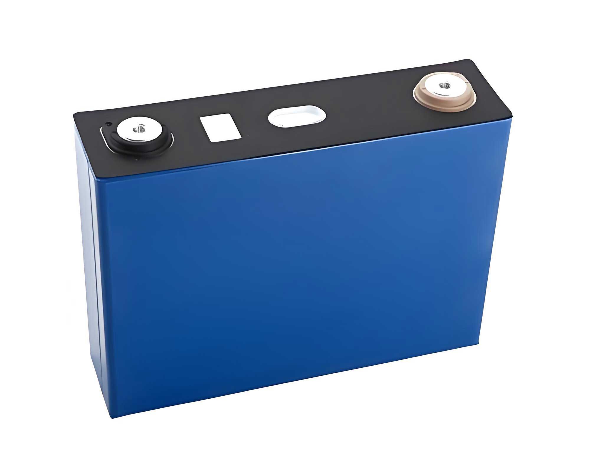
Parameter identification is performed using test data from a 271 Ah LiFePO4 cell used in marine battery packs. The process involves two main steps: determining the ohmic resistance \(R_0\) and fitting the hybrid model parameters \(B_1\) to \(B_4\) for charge and discharge separately.
1. Identifying Ohmic Resistance \(R_0\):
The internal resistance is derived from Hybrid Pulse Power Characteristic (HPPC) test data. The resistance is calculated at different SOC points using the voltage response to a pulsed discharge current \(I_L\), typically around 2C rate:
$$R_0 = \frac{U_0 – U_1}{I_L}$$
where \(U_0\) is the initial voltage and \(U_1\) is the voltage after the pulse. The calculated \(R_0\) values at various SOC levels are shown in the table below.
| SOC (%) | R₀ (mΩ) | SOC (%) | R₀ (mΩ) | SOC (%) | R₀ (mΩ) |
|---|---|---|---|---|---|
| 90 | 0.232 | 60 | 0.240 | 30 | 0.250 |
| 80 | 0.232 | 50 | 0.244 | 20 | 0.248 |
| 70 | 0.236 | 40 | 0.248 | 10 | 0.254 |
This data is then fitted to a 6th-order polynomial to obtain \(R_0\) as a continuous function of SOC, which is crucial for the model:
$$R_0(SOC_k) = -1.944SOC_k^6 + 5.545SOC_k^5 – 5.691SOC_k^4 + 2.5SOC_k^3 – 0.4262SOC_k^2 – 0.008788SOC_k + 0.2562$$
2. Fitting the Hybrid Model Parameters:
Due to the hysteresis effect, separate parameter sets are required for charge and discharge. Using constant-current charge and discharge test data, the parameters \(B_1\) to \(B_4\) and \(E_0\) are fitted via regression analysis, with \(R_0\) provided by the function above.
The finalized model for the charging process is:
$$V_k = 3.350 + 4.374 \frac{1}{SOC_k} – 27.72 \cdot SOC_k + 24.61 \ln(SOC_k) – 5.023 \ln(1-SOC_k) – i_k \cdot R_0(SOC_k)$$
The finalized model for the discharging process is:
$$V_k = 3.350 + 2.008 \frac{1}{SOC_k} – 77.36 \cdot SOC_k + 73.78 \ln(SOC_k) – 2.37 \ln(1-SOC_k) – i_k \cdot R_0(SOC_k)$$
The fitted curves show excellent agreement with the experimental data, confirming that this hybrid empirical model is sufficiently accurate for use in SOC estimation algorithm development.
Algorithms for SOC Estimation
SOC is defined as the ratio of remaining charge to nominal capacity:
$$SOC = \frac{Q_C}{Q_N}$$
Several methods exist for estimating SOC, each with strengths and weaknesses. The open-circuit voltage (OCV) method is simple but requires long rest periods and is not suitable for online estimation. The internal resistance method can be accurate but is difficult to model reliably. The ampere-hour (Ah) integration method is straightforward and widely used:
$$SOC(t) = SOC(t_0) – \frac{1}{Q_N} \int_{t_0}^{t} \eta i(\tau) d\tau$$
where \(\eta\) is the coulombic efficiency. However, it is an open-loop method highly sensitive to initial SOC error, current sensor drift, and capacity uncertainty, leading to accumulating errors over time.
For marine applications requiring high long-term accuracy and robustness, closed-loop estimation algorithms are superior. The Extended Kalman Filter (EKF) is a prominent algorithm in this category. It treats the SOC as an internal state of a dynamic system (the battery model) and uses a recursive predictor-corrector mechanism to optimally estimate the state based on noisy measurements (voltage, current).
The Extended Kalman Filter (EKF) Approach
The EKF is designed for nonlinear systems. It linearizes the system around the current state estimate at each time step. The state-space representation of the battery system is defined with SOC as the state and terminal voltage as the measurement.
1. State Equation (based on Ah integration):
$$SOC_{k+1} = SOC_k – \frac{\eta \Delta t}{Q_N} i_k + w_k$$
where \(w_k\) is the process noise, representing model inaccuracies.
2. Measurement Equation (based on the Hybrid Empirical Model):
$$V_k = f(SOC_k, i_k) + v_k$$
where \(f(SOC_k, i_k)\) is the nonlinear function described by the charging or discharging hybrid model, and \(v_k\) is the measurement noise (e.g., from voltage sensor).
3. EKF Algorithm Steps:
The algorithm proceeds recursively through two phases: Prediction and Update.
Prediction:
$$ \hat{SOC}_{k|k-1} = \hat{SOC}_{k-1|k-1} – \frac{\eta \Delta t}{Q_N} i_{k-1} $$
$$ P_{k|k-1} = A_{k-1} P_{k-1|k-1} A_{k-1}^T + Q $$
Here, \(P\) is the error covariance matrix, \(Q\) is the process noise covariance matrix, and \(A\) is the state transition Jacobian, which for our model is simply \(A_{k-1} = 1\).
Update:
First, linearize the measurement equation:
$$ C_k = \left. \frac{\partial f(SOC, i_k)}{\partial SOC} \right|_{SOC=\hat{SOC}_{k|k-1}} $$
This derivative is calculated analytically from the hybrid model equation. Then, compute the Kalman Gain \(K_k\), update the state estimate, and update the error covariance.
$$ K_k = P_{k|k-1} C_k^T (C_k P_{k|k-1} C_k^T + R)^{-1} $$
$$ \hat{SOC}_{k|k} = \hat{SOC}_{k|k-1} + K_k (V_{k,measured} – f(\hat{SOC}_{k|k-1}, i_k)) $$
$$ P_{k|k} = (1 – K_k C_k) P_{k|k-1} $$
Here, \(R\) is the measurement noise covariance matrix. The Kalman Gain optimally weights the correction from the measurement residual based on the confidence in the model (P) versus the confidence in the sensor (R).
The EKF’s strength lies in this feedback correction, which makes it robust to initial SOC error and capable of attenuating the effects of noise and slowly varying model errors over time. Its adaptability can be tuned via the \(Q\) and \(R\) matrices, making it suitable for the varying operational conditions of a marine LiFePO4 battery system.
Simulation of SOC Estimation Using EKF
A simulation platform is constructed in MATLAB/Simulink to validate the proposed methodology. The system comprises two main blocks: the high-fidelity Hybrid Empirical Battery Model (plant model) and the EKF estimator algorithm.
Simulation Setup:
The battery model is initialized with a true SOC of 0.5 (50%). A dynamic current profile consisting of 0.5C charge, discharge, and rest periods is applied. The EKF estimator is deliberately initialized with an incorrect SOC value of 0.6 (60%) to test its convergence capability. The process noise covariance \(Q\) and measurement noise covariance \(R\) are tuned to achieve a balance between estimation speed and stability.
Simulation Results and Analysis:
The simulation clearly demonstrates the power of the EKF algorithm. Despite the 10% initial error, the estimated SOC rapidly converges towards the true SOC value within approximately 20 seconds. After this initial transient, the estimation error remains bounded within a ±1% band throughout the subsequent charge-discharge cycles. The error exhibits a slight periodic variation corresponding to the current profile, which is expected as the linearized model has slight mismatches with the true nonlinear plant during high-current phases. However, the recursive nature of the EKF continuously corrects these small deviations, preventing any long-term drift. This performance starkly contrasts with the open-loop Ah integration method, where the initial 10% error would persist indefinitely.
The results underscore a critical insight: the accuracy of the EKF-based SOC estimation is heavily dependent on the precision of the underlying battery model. The well-fitted hybrid empirical model for the LiFePO4 battery provides the necessary nonlinear relationship \(f(SOC, i)\) that enables the EKF to make meaningful corrections. A poor model would lead to biased estimates regardless of the algorithmic sophistication.
Conclusion and Engineering Considerations
This exploration has detailed a methodological framework for high-accuracy SOC estimation for marine LiFePO4 battery systems, combining a refined Hybrid Empirical Model with an Extended Kalman Filter algorithm. The hybrid model successfully captures the unique voltage characteristics of the LiFePO4 chemistry, while the EKF provides a robust, closed-loop estimation mechanism that is resilient to initial error and sensor noise.
For practical marine engineering applications, several important factors must be addressed to transition from simulation to reliable onboard deployment. The performance of a LiFePO4 battery is significantly influenced by operational temperature. Future model development must incorporate thermal dependencies of parameters like \(R_0\), \(E_0\), and \(B_1\)-\(B_4\). Furthermore, battery aging leads to capacity fade (\(Q_N\) reduction) and internal resistance increase, which must be tracked and adapted online, possibly using dual or joint estimators. Finally, cell-to-cell variations within a large marine battery pack and the topology of the series-parallel connections necessitate strategies for estimating pack-level SOC from cell-level models, potentially involving representative cell monitoring or distributed estimation architectures.
In conclusion, the synergy of accurate electrochemical modeling and advanced recursive estimation algorithms like the EKF represents a powerful solution for marine battery management. As the computational power of embedded BMS controllers continues to grow, implementing such sophisticated algorithms becomes increasingly feasible. Continued research, supported by comprehensive data collection from real vessel operations, will further refine these models and algorithms, enhancing the safety, efficiency, and longevity of LiFePO4 battery systems in the global push towards greener maritime transportation.