
In the context of global efforts to address climate change, the goals of carbon peaking and carbon neutrality have driven a rapid transformation in energy systems. As renewable energy sources like wind and solar become increasingly integrated into the grid, the inherent variability and uncertainty of these sources pose significant challenges to grid stability. Energy storage systems, particularly those based on lithium iron phosphate batteries, have emerged as a critical solution for balancing supply and demand, providing frequency regulation, and enabling peak shaving. Among these, prefabricated cabin-type energy storage power stations offer modularity and scalability, making them widely deployed in utility-scale applications. However, the energy consumption of these stations during operation is a key factor affecting their overall efficiency and economic viability. This article delves into a comprehensive study on calculating the energy consumption of such stations, focusing on the losses inherent in the energy storage system itself and those from auxiliary equipment. By developing detailed methodologies and applying them to practical cases, I aim to provide a robust framework for engineers and planners to optimize energy storage performance.
The energy consumption of a prefabricated cabin lithium iron phosphate battery energy storage power station is influenced by multiple factors. First, the scale of the station determines the baseline energy loss, as larger installations involve more energy storage cells and associated equipment. Each energy storage cell contributes to overall losses through internal resistance during charge and discharge cycles. Second, the charge-discharge rate, often expressed in C-rate, significantly impacts the efficiency of the energy storage cells. Higher C-rates lead to greater resistive losses, reducing the round-trip efficiency. Third, the operational mode, such as participation in frequency response or arbitrage, affects the duration and intensity of cycles, thereby influencing cumulative energy consumption. Fourth, the cooling method, typically involving air conditioning systems in prefabricated cabins, plays a crucial role in maintaining optimal operating temperatures for the energy storage cells. The energy efficiency ratio (COP) of these cooling systems and their runtime directly contribute to auxiliary losses. Understanding these factors is essential for accurate energy consumption modeling.
To systematically calculate energy consumption, I divide the losses into two main categories: losses from the energy storage system itself and losses from auxiliary equipment operation. The energy storage system includes components like battery packs, DC cables, power conversion systems (PCS), transformers, and AC cables. Each component introduces efficiency losses that can be quantified. For the energy storage cells, the round-trip efficiency depends on the C-rate. For instance, at a 1 C-rate, the round-trip efficiency of lithium iron phosphate energy storage cells is typically no less than 92%, while at 0.5 C, it improves to at least 94%. This efficiency can be expressed as: $$\eta_e = f(C)$$ where $\eta_e$ is the battery efficiency and $C$ is the charge-discharge rate. The PCS efficiency varies with load and voltage, as shown in manufacturer data. A common approximation for PCS efficiency is 98% for both charge and discharge modes, but it can be modeled more precisely using curves. Transformer and cable losses are usually around 0.5% each. Thus, the overall round-trip efficiency for one complete charge-discharge cycle can be calculated as: $$\eta = \eta_e \times \eta_b \times \eta_{pc} \times \eta_{pd} \times \eta_x$$ where $\eta_b$ is transformer efficiency (e.g., 0.995), $\eta_{pc}$ and $\eta_{pd}$ are PCS charge and discharge efficiencies (e.g., 0.98 each), and $\eta_x$ accounts for other losses like cables (e.g., 0.995). Plugging in typical values for a 1 C-rate operation: $$\eta = 0.92 \times 0.995 \times 0.98 \times 0.98 \times 0.995 \approx 0.875$$ indicating a loss of about 12.5% per cycle.
The auxiliary equipment includes systems essential for station operation, such as air conditioning, lighting, battery management systems (BMS), fans, and security systems. Among these, air conditioning is the most significant consumer, as it regulates the temperature within the prefabricated cabin to ensure the energy storage cells operate within safe and efficient ranges. The energy consumption of auxiliary devices depends on operational states—running during charge-discharge cycles and idle during standby. For example, air conditioning may run at full cooling capacity during active cycles and switch to low-power internal circulation otherwise. To estimate auxiliary losses, I compile data from typical installations. The table below summarizes the power consumption of key auxiliary devices in a prefabricated cabin energy storage station.
| Equipment Type | Device | Power (kW) | Quantity | Total Power (kW) |
|---|---|---|---|---|
| Battery Cabin | Industrial Air Conditioner | 20 | 2 | 40 |
| Lighting | 1.5 | 1 | 1.5 | |
| BMS and Fans | 3 | 1 | 3 | |
| UPS | 3 | 1 | 3 | |
| Emergency Lighting | 1.2 | 1 | 1.2 | |
| Other Cabins | Air Conditioners | 3 | 4 | 12 |
| Transformers & Fans | Varies | Multiple | ~5 | |
| Lighting | 1.5 | 3 | 4.5 | |
| Total Auxiliary Power | Approx. 70 kW during peak operation | ~70 | ||
The energy consumption from auxiliary devices is highly dependent on runtime. For a station operating in a one-cycle-per-day mode (e.g., 2 hours of charge-discharge), air conditioning might run for 4 hours in summer to dissipate heat generated by the energy storage cells, consuming significant energy. In winter, heating may add to the load. The daily auxiliary energy consumption $E_{aux}$ can be estimated as: $$E_{aux} = \sum (P_i \times t_i)$$ where $P_i$ is the power of device $i$ and $t_i$ is its runtime. For instance, if air conditioning runs at 40 kW for 4 hours and other devices at 5 kW for 24 hours (with a simultaneity factor of 0.5), then $E_{aux} = (40 \times 4) + (5 \times 24 \times 0.5) = 160 + 60 = 220 \text{ kWh}$. This highlights the importance of optimizing auxiliary systems to reduce overall energy consumption.
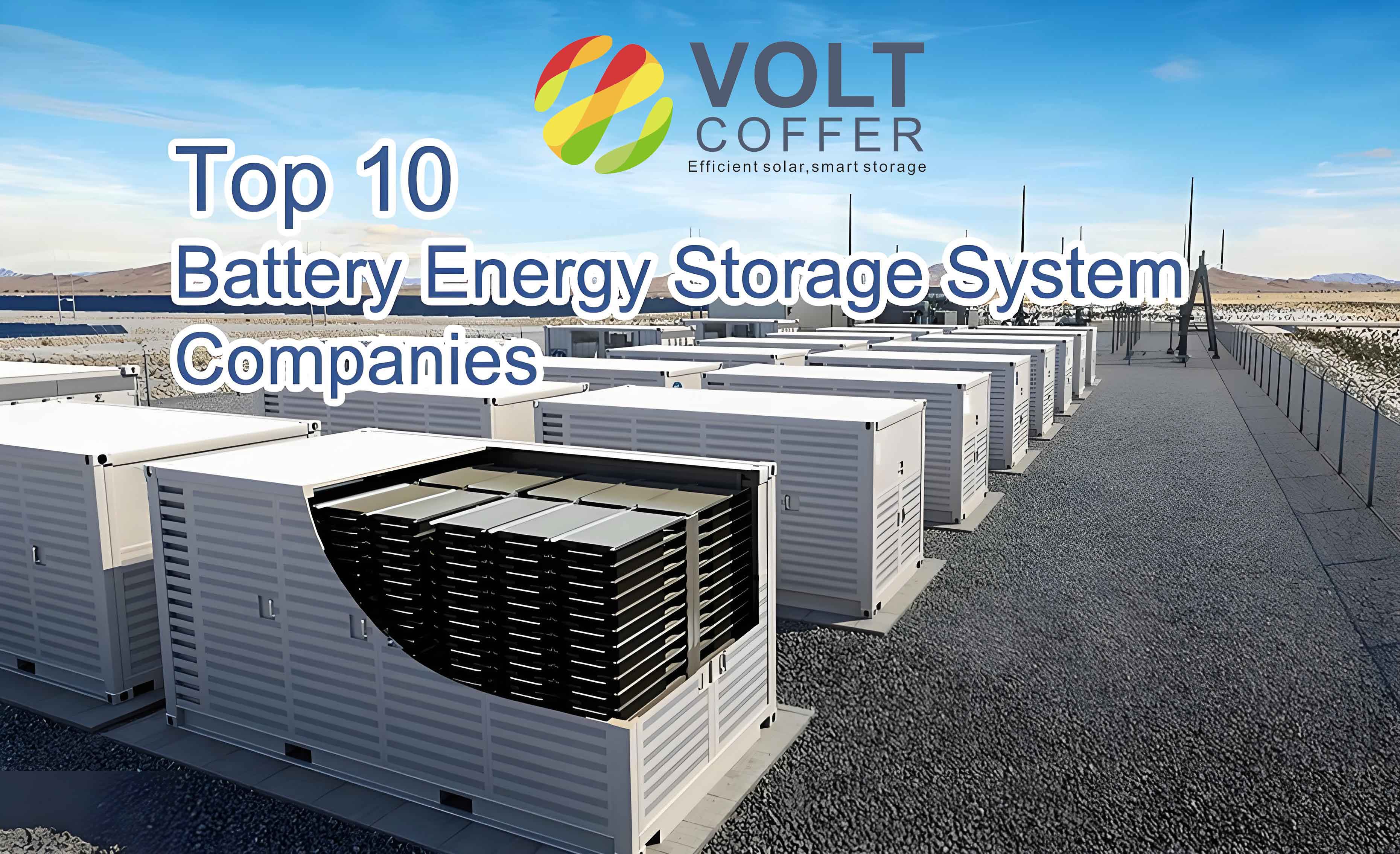
To validate the methodology, I analyze a case study of a 2 MW/2 MWh energy storage battery cabin. This cabin is equipped with lithium iron phosphate energy storage cells configured in a 240S16P arrangement, meaning 240 cells in series and 16 in parallel, providing the desired voltage and capacity. The energy storage cells have a rated cycle life of over 5,000 cycles at 1 C and 25°C, with a system conversion efficiency of at least 92%. The cabin includes two industrial air conditioners, each with a maximum cooling power of 17.5 kW and heating power of 15 kW. During operation, the energy storage cells undergo charge-discharge cycles at 1 C, and the auxiliary devices operate as per the station’s control strategy.
The theoretical energy consumption for one full charge-discharge cycle can be calculated using the efficiency formula. Assuming a charge input of 2 MWh, the discharge output is: $$E_{out} = E_{in} \times \eta = 2000 \text{ kWh} \times 0.875 = 1750 \text{ kWh}$$ Thus, the energy loss in the storage system is: $$E_{loss,system} = 2000 – 1750 = 250 \text{ kWh}$$ However, this loss manifests as heat generated by the energy storage cells. In an adiabatic assumption, this heat must be removed by the air conditioning system. The air conditioners have a total cooling capacity of 80 kW (40 kW each from power consumption and COP effects). To dissipate 250 kWh of heat, the required runtime is: $$t_{cool} = \frac{250 \text{ kWh}}{80 \text{ kW}} = 3.125 \text{ hours}$$ This theoretical runtime suggests that auxiliary energy consumption for cooling would be: $$E_{cool} = 40 \text{ kW} \times 3.125 = 125 \text{ kWh}$$ Adding other auxiliary devices (e.g., 60 kWh per day), the total auxiliary consumption becomes approximately 185 kWh. Compared to field test results of 280 kWh per day, there is a discrepancy, indicating that real-world factors like non-adiabatic conditions, seasonal variations, and control strategies play a role.
Field tests on the 2 MW/2 MWh cabin revealed that in summer, air conditioning ran for about 4 hours at full cooling, consuming 140 kWh, while in idle mode, it used 80 kWh over 20 hours, totaling 220 kWh for air conditioning alone. Other devices added around 60 kWh, leading to 280 kWh daily. This exceeds the theoretical calculation due to additional heat ingress from the environment and inefficiencies in the cooling system. The energy storage cells’ heat generation is not perfectly coupled with air conditioning removal, and factors like solar radiation on the cabin walls increase the thermal load. Moreover, the battery management system may activate cooling preemptively to protect the energy storage cells, extending runtime. These insights underscore the need for dynamic models that account for real-time thermal interactions.
To refine the energy consumption calculation, I propose incorporating more detailed sub-models. For the energy storage cells, the efficiency can be expressed as a function of state-of-charge (SOC), temperature, and C-rate: $$\eta_e = \eta_0 – k_1 \cdot C – k_2 \cdot |T – T_{opt}|$$ where $\eta_0$ is the base efficiency, $k_1$ and $k_2$ are coefficients, $C$ is the C-rate, and $T$ is the cell temperature. This allows for granular adjustments based on operational data. Similarly, PCS efficiency can be modeled using polynomial fits from manufacturer curves: $$\eta_{pc} = a_0 + a_1 \cdot L + a_2 \cdot L^2$$ where $L$ is the load ratio and $a_i$ are coefficients. For auxiliary systems, the air conditioning energy consumption can be tied directly to the heat balance of the cabin: $$Q_{gen} = E_{loss,system} + Q_{env}$$ where $Q_{gen}$ is the total heat to be removed, $E_{loss,system}$ is from battery losses, and $Q_{env}$ is environmental heat gain. The air conditioning energy is then: $$E_{ac} = \frac{Q_{gen}}{COP \cdot \eta_{ac}}$$ with COP as the coefficient of performance and $\eta_{ac}$ as air conditioner efficiency.
To illustrate the impact of different parameters, I present a series of tables and formulas. Below is a table showing round-trip efficiency variations with C-rate for lithium iron phosphate energy storage cells.
| C-rate | Battery Round-trip Efficiency ($\eta_e$) | Overall System Efficiency ($\eta$) | Energy Loss per Cycle for 2 MWh Input (kWh) |
|---|---|---|---|
| 1.0 | 0.92 | 0.875 | 250 |
| 0.5 | 0.94 | 0.894 | 212 |
| 0.25 | 0.96 | 0.913 | 174 |
This table demonstrates that lower C-rates improve efficiency, reducing energy consumption. However, operational requirements may dictate higher C-rates for rapid response, so a trade-off exists. Additionally, the energy consumption of auxiliary devices varies with season. The next table summarizes estimated daily auxiliary energy for different seasons, assuming a one-cycle operation.
| Season | Air Conditioning Runtime (hours) | Air Conditioning Energy (kWh) | Other Auxiliary Energy (kWh) | Total Auxiliary Energy (kWh) |
|---|---|---|---|---|
| Summer | 4 | 140 | 60 | 200 |
| Winter | 3 (cooling) + 2 (heating) | 125 | 60 | 185 |
| Spring/Autumn | 2 | 70 | 60 | 130 |
These values are illustrative and based on typical conditions; actual data may vary. To achieve a comprehensive energy consumption model, I integrate the system and auxiliary losses. The total daily energy consumption $E_{total}$ for a station with $n$ cycles per day is: $$E_{total} = n \cdot E_{loss,system} + E_{aux}$$ For the case study with $n=1$, $E_{loss,system} = 250 \text{ kWh}$, and $E_{aux} = 280 \text{ kWh}$, we get $E_{total} = 530 \text{ kWh}$. This represents the energy drawn from the grid that does not contribute to useful output, highlighting areas for optimization.
The role of the energy storage cell is central to these calculations. Each energy storage cell within the battery pack contributes to losses through internal resistance, which generates heat during charge and discharge. The heat generation per cell can be approximated by: $$Q_{cell} = I^2 \cdot R \cdot t$$ where $I$ is the current, $R$ is the internal resistance, and $t$ is the time. For a pack with thousands of energy storage cells, the cumulative heat is substantial, driving cooling needs. Advanced thermal management systems, such as liquid cooling or phase-change materials, can reduce auxiliary energy consumption by improving heat transfer efficiency. However, in prefabricated cabins, air cooling remains common due to cost and simplicity. Optimizing the layout of energy storage cells within the cabin to enhance natural convection can also lower cooling loads.
Another factor is the aging of energy storage cells. Over time, the internal resistance of lithium iron phosphate energy storage cells increases, leading to higher losses and reduced efficiency. This aging effect can be modeled by incorporating a degradation factor into the efficiency equation: $$\eta_e(t) = \eta_{e,0} \cdot e^{-\lambda t}$$ where $\lambda$ is the degradation rate and $t$ is time or cycle count. This adds complexity to long-term energy consumption forecasts. For example, after 1,000 cycles, the efficiency might drop by 2-3%, increasing energy consumption proportionally. Therefore, maintenance schedules and cell replacement strategies should consider these dynamics.
In practice, energy consumption statistics for storage stations require long-term monitoring. Field tests provide snapshots, but continuous data collection is needed to account for seasonal variations, load profiles, and equipment performance. I recommend installing smart meters on auxiliary circuits and integrating data with energy management systems. This allows for real-time optimization, such as adjusting air conditioning setpoints based on forecasted weather or scheduling cycles during cooler periods. Moreover, benchmarking against theoretical models helps identify anomalies, like faulty energy storage cells or inefficient cooling, enabling proactive maintenance.
To further elaborate on the methodology, I derive formulas for specific components. For DC and AC cables, the power loss $P_{cable}$ is: $$P_{cable} = I^2 \cdot R_{cable}$$ where $R_{cable}$ is the resistance. Over a cycle time $t_{cycle}$, the energy loss is: $$E_{cable} = P_{cable} \cdot t_{cycle}$$ For transformers, the loss includes no-load and load losses, often provided by manufacturers. A simplified approach uses an efficiency value, but for precision, the following can be used: $$E_{transformer} = P_{no-load} \cdot t_{total} + P_{load} \cdot \left( \frac{I}{I_{rated}} \right)^2 \cdot t_{cycle}$$ where $t_{total}$ is the total operational time. These detailed calculations improve accuracy, especially for large stations.
Regarding auxiliary devices, the battery management system (BMS) is essential for monitoring the energy storage cells. Its power consumption is relatively low but constant. BMS algorithms that optimize charge profiles can reduce energy losses in the cells. For instance, by avoiding high C-rates when possible, the BMS can enhance overall efficiency. Similarly, variable-speed drives for fans and pumps in cooling systems can match airflow to thermal loads, saving energy. The energy consumption of these devices can be modeled with power-speed curves: $$P_{fan} = P_{rated} \cdot \left( \frac{N}{N_{rated}} \right)^3$$ where $N$ is the fan speed. Integrating such models into station design can lead to significant savings.
In conclusion, calculating the energy consumption of prefabricated cabin lithium iron phosphate battery energy storage stations involves a multifaceted approach. By dissecting losses into system and auxiliary categories, and employing detailed formulas and tables, I have developed a framework that captures key factors like C-rate, operational mode, and cooling requirements. The case study of a 2 MW/2 MWh cabin demonstrates the application of this framework, revealing discrepancies between theoretical and field results that underscore the importance of real-world data. The energy storage cell is at the heart of these calculations, with its efficiency dictating much of the loss. Moving forward, continuous monitoring and advanced thermal management will be crucial for minimizing energy consumption, thereby enhancing the sustainability and cost-effectiveness of energy storage systems. This research provides a valuable reference for engineers seeking to optimize such stations in the evolving energy landscape.