
The stability of modern power systems faces significant challenges due to the increasing integration of renewable energy sources, characterized by inherent intermittency and unpredictability. These characteristics exacerbate the inherent limitations of traditional frequency regulation units, such as slow response times. Energy storage batteries offer a compelling solution with their rapid response, high power density, and flexible controllability. This article proposes an advanced control strategy for energy storage battery participation in primary frequency regulation, which strategically leverages ultra-short-term load forecasting to optimize both frequency control performance and the long-term operational health of the battery itself.
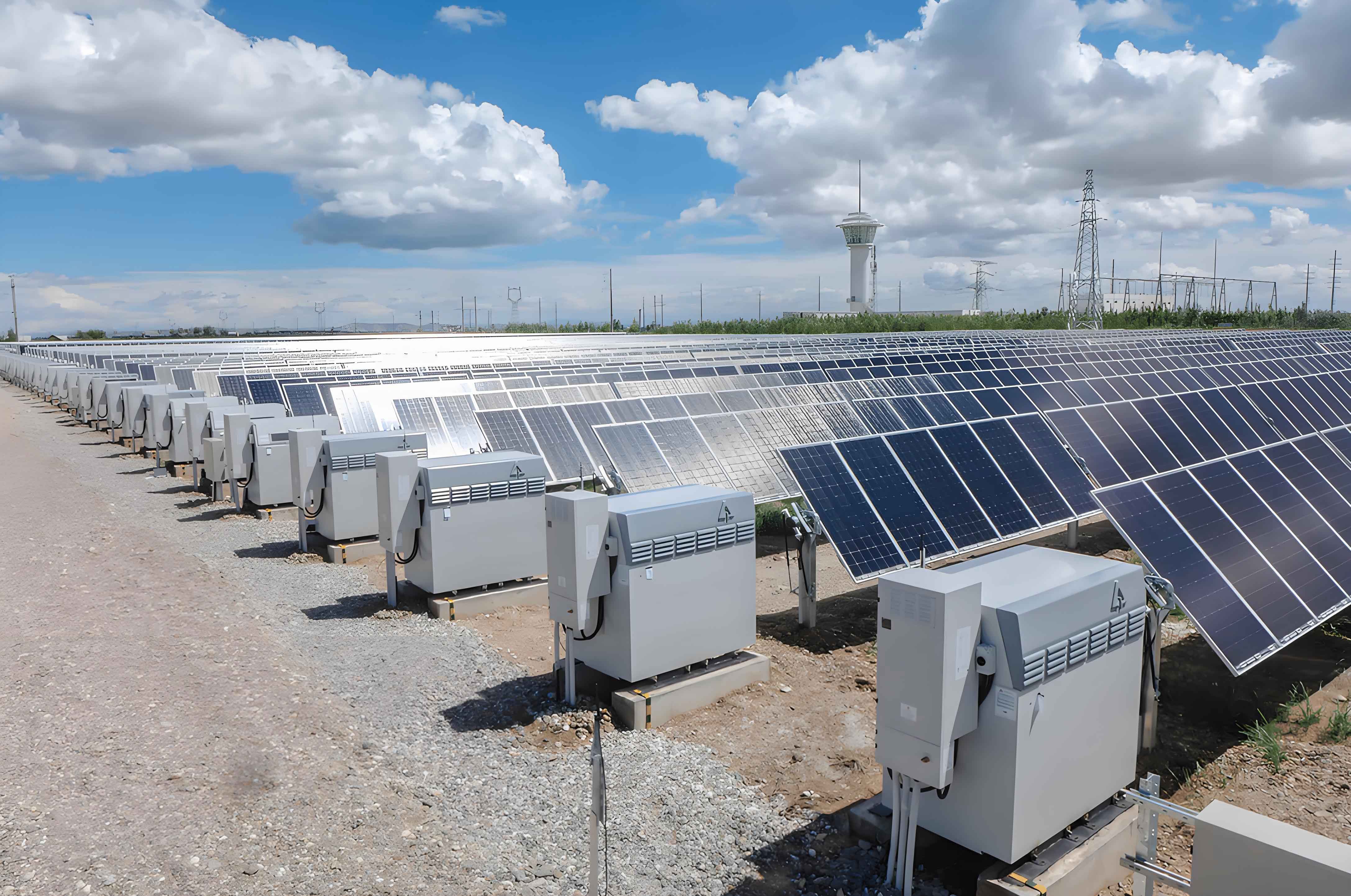
The core objective is to design an output strategy that not only improves the system’s dynamic frequency response but also proactively manages the state-of-charge (SOC) of the energy storage battery. This is achieved by using forecasted load trends to anticipate regulation demands and adjust the battery’s readiness state accordingly.
1. System Modeling for Frequency Regulation with Energy Storage
To analyze the dynamic behavior, a regional power grid model incorporating traditional generation and an energy storage battery is established. The model represents the collective dynamics of system components for frequency regulation studies.
The frequency deviation $\Delta f(s)$ resulting from a load disturbance $\Delta P_L(s)$ is governed by the swing equation and the combined response of traditional generators and the energy storage battery. The block diagram representation captures the interactions, where the total power imbalance is compensated by the sum of traditional generator output $\Delta P_G(s)$ and energy storage battery output $\Delta P_b(s)$.
The transfer function for the traditional thermal generator is typically represented as a combination of a governor and a turbine model:
$$ G_g(s) = G_{gov}(s) \cdot G_{en}(s) = \frac{1}{1+sT_g} \cdot \frac{1+sF_{HP}T_{RH}}{(1+sT_{CH})(1+sT_{RH})} $$
where $T_g$, $T_{CH}$, $T_{RH}$ are the governor, turbine, and reheater time constants, respectively, and $F_{HP}$ is the high-pressure power fraction.
The energy storage battery is modeled with a first-order lag to represent its power conversion dynamics:
$$ G_b(s) = \frac{1}{1+sT_b} $$
where $T_b$ is the battery time constant, typically much smaller than traditional generator time constants, highlighting its fast response capability.
The system frequency dynamics are described by:
$$ \Delta f(s) = \frac{1}{Ms + D} \left[ \Delta P_L(s) – \Delta P_G(s) – \Delta P_b(s) \right] $$
where $M$ is the system inertia constant and $D$ is the load damping coefficient. The traditional generator output responds to frequency deviation via its droop characteristic $K_g$, while the energy storage battery output is determined by the control strategy discussed in the next section.
2. Control Strategy Design for the Energy Storage Battery
The proposed control strategy for the energy storage battery operates in two distinct modes: the Frequency Regulation Mode and the SOC Recovery Mode. The strategy seamlessly switches between these modes based on system frequency and information from load forecasting.
2.1 Adaptive Output Strategy During Frequency Regulation
During periods of significant frequency deviation (outside a defined deadband), the energy storage battery operates in the Frequency Regulation Mode using a virtual droop control principle. The output power is proportional to the frequency deviation:
$$ \Delta P_b = K \cdot \Delta f $$
where $K$ is the virtual droop coefficient or unit regulating power.
A fixed $K$ value can lead to rapid depletion or saturation of the energy storage battery’s SOC during prolonged disturbances, impairing its future availability and potentially harming battery health. Therefore, an adaptive strategy is proposed where $K$ varies dynamically with the real-time SOC of the energy storage battery. This creates an “S-curve” relationship, reducing the battery’s output when its SOC is extremely low or high to preserve capacity, while allowing full output when SOC is in a healthy mid-range.
The adaptive coefficients for discharge ($K_{disch}$) and charge ($K_{ch}$) are defined by piecewise functions:
For discharging ($\Delta f < 0$):
$$
K_{disch} =
\begin{cases}
0 & 0 < S_{SOC} < S_{SOC,min} \\[6pt]
\dfrac{K_{max} P_0 e^{\,n\frac{S_{SOC}-0.1}{0.35}} }{K_{max} + P_0 \left( e^{\,n\frac{S_{SOC}-0.1}{0.35}} – 1 \right)} & S_{SOC,low} \le S_{SOC} \le S_{SOC,high} \\[12pt]
K_{max} & S_{SOC,high} < S_{SOC} < S_{SOC,max}
\end{cases}
$$
For charging ($\Delta f > 0$):
$$
K_{ch} =
\begin{cases}
K_{max} & 0 < S_{SOC} < S_{SOC,min} \\[6pt]
\dfrac{K_{max} P_0 e^{\,n\frac{0.9-S_{SOC}}{0.35}} }{K_{max} + P_0 \left( e^{\,n\frac{0.9-S_{SOC}}{0.35}} – 1 \right)} & S_{SOC,low} \le S_{SOC} \le S_{SOC,high} \\[12pt]
0 & S_{SOC,high} < S_{SOC} < S_{SOC,max}
\end{cases}
$$
Here, $K_{max}$ is the maximum virtual unit regulating power, $P_0$ is the rated power of the energy storage battery, $n$ is a curve shaping coefficient (e.g., $n=15$), and $S_{SOC,min}, S_{SOC,low}, S_{SOC,high}, S_{SOC,max}$ are threshold SOC values (e.g., 0.1, 0.45, 0.55, 0.9).
2.2 Dynamic SOC Recovery Strategy Using Bi-level Fuzzy Control
When the system frequency is within the normal deadband, the energy storage battery switches to the SOC Recovery Mode. The goal is to adjust its SOC to an optimal target level in preparation for the next anticipated frequency regulation event. This target is not fixed at 0.5 but is dynamically set based on ultra-short-term load forecasting.
The reference power change for the upcoming period, $\Delta P_{ref}$, is derived from the forecast:
$$ \Delta P_{ref} = \Delta P_L + \Delta P_T – \Delta P_{NLD} $$
where $\Delta P_L$ is the forecasted load change, $\Delta P_T$ is the scheduled tie-line power change, and $\Delta P_{NLD}$ is the non-regulating generation.
First-Level Fuzzy Controller (Target SOC Setting): This controller determines the dynamic SOC benchmark ($S_{SOC}^*$) for the next regulation period based on $\Delta P_{ref}$. The rule is: a large positive $\Delta P_{ref}$ (implying future need for discharge) warrants a high target SOC; a large negative $\Delta P_{ref}$ warrants a low target SOC; near-zero $\Delta P_{ref}$ warrants a target SOC of 0.5.
The fuzzy rules for the first level are summarized below:
| Input: $\Delta P_{ref}$ | Output: $S_{SOC}^*$ |
|---|---|
| NB (Negative Big) | NB (e.g., 0.2) |
| NS (Negative Small) | NS (e.g., 0.35) |
| ZO (Zero) | ZO (0.5) |
| PS (Positive Small) | PS (e.g., 0.65) |
| PB (Positive Big) | PB (e.g., 0.8) |
Second-Level Fuzzy Controller (Recovery Power Control): This controller determines the actual charge/discharge power $P_b$ during the recovery period. It has two inputs: the SOC error $\Delta S_{SOC} = S_{SOC}^* – S_{SOC}(t)$ and the current frequency deviation $\Delta f$. Its output is the recovery power. The logic ensures recovery actions do not push the frequency out of its deadband. For example, if $\Delta S_{SOC}$ is positive (need to charge) and $\Delta f$ is slightly positive (frequency above nominal, allowing gentle charging), then a positive $P_b$ (charging) is applied.
The fuzzy rule surface for the second-level controller is conceptualized as follows:
| $\Delta f$ / $\Delta S_{SOC}$ | NB | NS | ZO | PS | PB |
|---|---|---|---|---|---|
| NB | NB | NB | ZO | ZO | ZO |
| NS | NB | NB | ZO | ZO | ZO |
| ZO | NS | NS | ZO | PS | PS |
| PS | ZO | ZO | ZO | PB | PB |
| PB | ZO | ZO | ZO | PB | PB |
(Where NB, NS, ZO, PS, PB for output $P_b$ correspond to levels of discharge/charge power).
3. Performance Evaluation Metrics
To quantitatively assess the proposed strategy, key performance indicators (KPIs) are defined for both frequency regulation effect and energy storage battery health.
Frequency Regulation KPIs:
For a frequency event with initial time $t_0$, maximum deviation time $t_m$, and settling time $t_s$:
- Maximum Frequency Deviation: $\Delta f_m = \Delta f(t_m)$
- Frequency Nadir/Roocoof Rate: $V_m = (\Delta f_0 – \Delta f_m) / (t_m – t_0)$
- Frequency Recovery Rate: $V_r = (\Delta f_s – \Delta f_m) / (t_s – t_m)$
Superior performance is indicated by smaller $|\Delta f_m|$ and $|V_m|$, and a larger $V_r$.
Energy Storage Battery SOC Health KPI:
A health index $H$ is defined as the root-mean-square deviation of the operating SOC from the nominal 0.5 level over a time period with $k$ samples:
$$ H = \sqrt{ \frac{1}{k} \sum_{i=1}^{k} \left( S_{SOC,i} – 0.5 \right)^2 } $$
A lower $H$ value indicates the energy storage battery operates closer to its nominal, healthy SOC mid-point on average, which is beneficial for longevity.
4. Case Study and Comparative Analysis
A simulation study is conducted on a regional grid model with a 100 MW base. An energy storage battery with a capacity of 1 MW / 0.25 MWh (1% of base power) is added. The proposed Dynamic SOC Benchmark strategy is compared against three benchmarks:
- No Storage: Baseline with only traditional generators.
- Fixed-K Strategy: Energy storage battery uses a constant, maximum $K$ value.
- 0.5-SOC Benchmark Strategy: Energy storage battery always recovers SOC to 0.5 during idle times, without forecasting.
Key simulation parameters are listed below:
| Parameter | Value | Parameter | Value |
|---|---|---|---|
| Power Base | 100 MW | Governor Time Const. $T_g$ | 0.08 s |
| Frequency Base | 50 Hz | Battery Time Const. $T_b$ | 0.01 s |
| System Inertia $M$ | 5 s | Gen. Droop $K_g$ | 10 p.u. |
| Load Damping $D$ | 1 p.u. | Max. Battery Droop $K_{b,max}$ | 24 p.u. |
| Battery Capacity | 0.25 MWh | Frequency Deadband | $\pm$0.00066 p.u. |
4.1 Case 1: Step Load Increase (0.02 p.u.)
The system response to a significant step disturbance is simulated. The results demonstrate the critical role of the energy storage battery in improving frequency stability.
The proposed Dynamic SOC Benchmark strategy effectively reduces the maximum frequency deviation ($\Delta f_m$) compared to all other strategies. While the Fixed-K strategy shows a slightly faster initial rate of frequency decline ($V_m$), its aggressive use of the energy storage battery leads to complete depletion of the battery SOC shortly after the event. This leaves the system vulnerable to subsequent disturbances. In contrast, the proposed strategy maintains a reasonable SOC reserve.
The 0.5-SOC Benchmark strategy also depletes the battery but performs worse in minimizing $\Delta f_m$ than the proposed strategy because it does not pre-charge the battery based on the forecasted need for increased generation.
| Strategy | $\Delta f_m$ (10$^{-4}$ p.u.) | $V_m$ (10$^{-5}$ p.u./s) | $V_r$ (10$^{-4}$ p.u./s) | SOC Post-Event |
|---|---|---|---|---|
| No Storage | 2.80 | 1.400 | 0.300 | N/A |
| Fixed-K | 2.30 | 0.400 | 0.200 | Depleted (0.1) |
| 0.5-SOC Benchmark | 1.80 | 0.900 | 0.005 | Low |
| Proposed (Dynamic SOC) | 1.25 | 0.625 | 0.005 | Moderate (~0.4) |
4.2 Case 2: Continuous Load Fluctuations
A one-hour realistic load profile is used, with the ultra-short-term forecast assumed perfect for a 1-hour horizon, updated every minute. The simulation involves three cycles, each with a regulation period ($J_1, J_2, J_3$) and a recovery period ($I_1, I_2, I_3$).
The advantages of the proposed strategy are more pronounced over this extended, dynamic scenario. The Fixed-K strategy again provides good initial frequency control but exhausts the energy storage battery capacity before the end of the simulation, causing a severe frequency jump when the battery disconnects at its SOC limit. The 0.5-SOC Benchmark strategy often fails to prepare adequately for upcoming regulation needs, leading to larger frequency deviations.
The proposed Dynamic SOC Benchmark strategy, by proactively adjusting the target SOC based on the forecast, consistently maintains a better SOC buffer. It successfully pre-charges the battery before periods of expected high load and pre-discharges before periods of expected low load. This results in more robust frequency support throughout the entire period and a significantly better SOC health index $H$.
| Strategy | $\Delta f_m$ in $J_1$ | $\Delta f_m$ in $J_2$ | $\Delta f_m$ in $J_3$ | SOC Health Index $H$ |
|---|---|---|---|---|
| No Storage | -0.875 | 1.07 | -0.875 | N/A |
| Fixed-K | -0.375 | 0.55 | -1.275* | 0.2488 |
| 0.5-SOC Benchmark | -0.625 | 1.68 | -1.850 | 0.1934 |
| Proposed (Dynamic SOC) | -0.625 | 0.55 | -0.725 | 0.1884 |
*Battery depleted during $J_3$, causing a frequency collapse.
5. Conclusion
This article presents a novel, integrated control strategy for energy storage battery participation in primary frequency regulation. The strategy’s innovation lies in its two-fold adaptive approach: an SOC-aware virtual droop control during active regulation, and a forecast-guided, fuzzy logic-based SOC recovery mechanism during idle periods. The integration of ultra-short-term load forecasting provides crucial foresight, allowing the energy storage battery to strategically position its SOC in anticipation of future regulation demands.
Simulation results under both step and continuous load disturbances confirm the effectiveness of the proposed strategy. Compared to a fixed-gain strategy, it significantly enhances the sustainability of frequency support by preventing premature energy depletion of the energy storage battery. Compared to a simple 0.5-SOC recovery strategy, it improves both the quality of frequency regulation and the long-term health of the energy storage battery, as measured by a lower SOC health index $H$.
In summary, the coordinated use of adaptive droop control and predictive SOC management enables the energy storage battery to serve as a highly reliable and sustainable resource for grid frequency stabilization. Future work will focus on optimizing the sizing of the energy storage battery considering economic factors under this strategy, and incorporating additional real-world constraints such as generator ramping rates and system reserve status.