
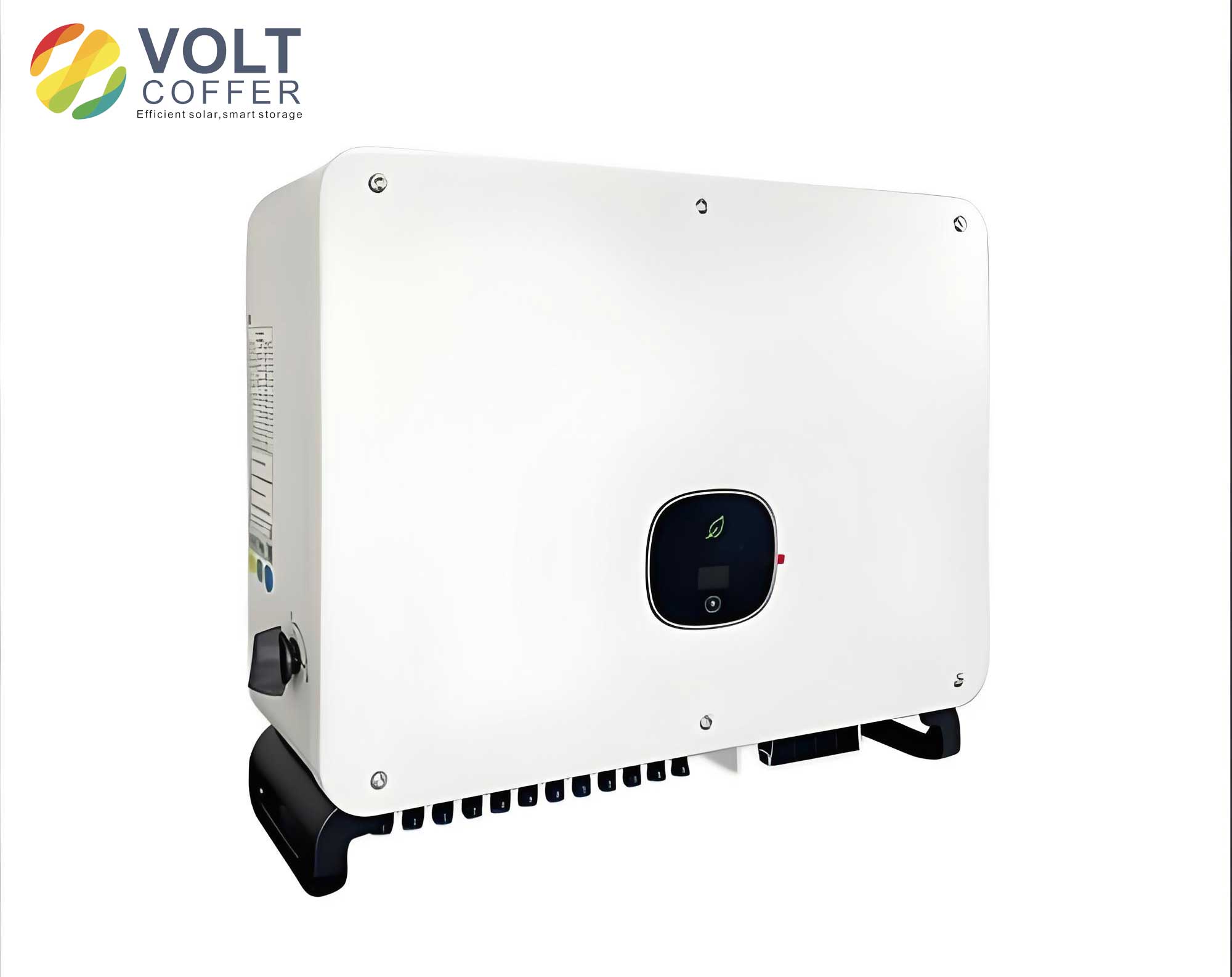
The global imperative for sustainable and clean energy has propelled solar photovoltaic (PV) technology to the forefront of power generation. As a core component of any grid-connected PV system, the performance and reliability of the utility interactive inverter are paramount. This device performs the critical function of converting direct current (DC) from solar panels into grid-compliant alternating current (AC). The control technology governing this utility interactive inverter directly determines the quality of the injected power, the stability of the grid connection, and the overall efficiency of the energy harvest. This article delves into advanced control methodologies, focusing on a dual-loop control strategy based on Sinusoidal Pulse Width Modulation (SPWM) to achieve high-performance, stable, and efficient operation of solar PV systems.
The primary objective of a utility interactive inverter is to inject a sinusoidal current into the utility grid that is perfectly synchronized in frequency and phase with the grid voltage, typically at unity power factor. This ensures maximum real power transfer and minimizes reactive power flow, which is crucial for grid stability and power quality. The core challenge lies in accurately tracking the grid’s sinusoidal reference amidst disturbances, grid impedance variations, and non-ideal component behaviors.
Fundamentally, control methods for the output current of a utility interactive inverter can be categorized into two main approaches:
| Control Method | Principle | Advantages | Disadvantages |
|---|---|---|---|
| Direct Current Control | Uses the calculated or sensed AC current as a feedback signal to directly force the inverter output current to follow its reference. | Fast dynamic response, simple principle, less dependent on system parameters. | Requires high-bandwidth current sensors. |
| Indirect Current Control (Voltage Control) | Controls the AC output voltage amplitude and phase to indirectly regulate the current flowing into the grid voltage source. | Can eliminate the need for grid current sensors. | Slower response, complex control design, prone to DC offset in current. |
For high-performance applications, direct current control, often implemented with Pulse Width Modulation (PWM) techniques like SPWM, is predominant. The combination of an outer voltage loop and an inner current loop (dual-loop control) provides excellent dynamic performance and output waveform quality. This forms the basis of our detailed analysis.
The most common power stage for a single-phase utility interactive inverter is the full-bridge (H-bridge) topology. The DC-link voltage $V_{dc}$ is switched by the four power devices (S1-S4) to generate a bipolar PWM voltage $v_{ab}$ at the bridge terminals. An inductor $L$ serves as the main filter component, smoothing the PWM voltage into a sinusoidal current $i_L$. The key differential equation describing this AC side is:
$$ v_{ab}(t) = v_{net}(t) + L \frac{di_L(t)}{dt} + R_L i_L(t) $$
where $v_{net}$ is the grid voltage and $R_L$ is the equivalent resistance of the inductor and wiring.
Transforming this into the Laplace domain provides the plant model for controller design. The transfer function from the inverter bridge output voltage $V_{ab}(s)$ to the grid current $I_L(s)$, considering the grid voltage as a disturbance, is:
$$ G_p(s) = \frac{I_L(s)}{V_{ab}(s)} = \frac{1}{sL + R_L} $$
The PWM bridge itself introduces a small time delay, which can be approximated as a first-order lag with a time constant $T_P$ equal to the PWM switching period. Its transfer function is:
$$ G_{PWM}(s) = \frac{K_{PWM}}{T_P s + 1} $$
where $K_{PWM}$ is the gain of the bridge (typically $V_{dc}$ / carrier amplitude).
The complete uncontrolled open-loop transfer function of the system, including the PWM delay and a feedback gain $a$ (from current sensor and signal conditioning), becomes:
$$ G_{ol,uncontrolled}(s) = a \cdot G_{PWM}(s) \cdot G_p(s) = \frac{a \cdot K_{PWM}}{(T_P s + 1)(sL + R_L)} $$
An analysis of the step response of this open-loop system reveals poor stability, a slow response, and a significant steady-state error, necessitating the design of a closed-loop controller.
To achieve zero steady-state error for a DC reference and provide good dynamic tracking for an AC sinusoidal reference, a Proportional-Integral (PI) controller is a standard choice. The transfer function of a PI controller is:
$$ G_{PI}(s) = K_P + \frac{K_I}{s} = \frac{K_P s + K_I}{s} $$
where $K_P$ is the proportional gain and $K_I$ is the integral gain.
We employ the “Second-Order Optimum” (or modulus optimum) method for tuning. The goal is to cancel the dominant plant pole (from the inductor) with the PI zero and set the open-loop crossover frequency for desired dynamics. The closed-loop system with the PI controller and plant has the following structure. The open-loop transfer function after zero-pole cancellation ($K_I/K_P = R_L/L$) is:
$$ G_{ol}(s) = G_{PI}(s) \cdot G_{PWM}(s) \cdot G_p(s) \approx \frac{a \cdot K_{PWM} \cdot K_P}{s \cdot L \cdot (T_P s + 1)} $$
For a second-order optimum system, we set the open-loop gain to achieve a phase margin near 65°. A standard design sets:
$$ a \cdot K_{PWM} \cdot K_P / L = 1 / (2 T_P) $$
This yields the following closed-loop transfer function, which approximates a well-damped second-order system:
$$ G_{cl}(s) \approx \frac{1}{2 T_P^2 s^2 + 2 T_P s + 1} $$
Using typical values (L=4mH, R_L=0.5Ω, T_P=100µs for 10kHz switching, a=0.05 V/A, K_PWM=200), we can calculate the PI parameters.
| Parameter | Symbol | Value | Note |
|---|---|---|---|
| Integral Gain | $K_I$ | $K_P \cdot (R_L / L) = 62.5$ | Sets PI zero to cancel plant pole. |
| Proportional Gain | $K_P$ | $L / (2 a K_{PWM} T_P) = 0.2$ | From modulus optimum criterion. |
| Phase Margin | PM | > 65° | Ensures stability and damping. |
| Crossover Frequency | $f_c$ | ~ 720 Hz | Indicates control bandwidth. |
While the PI controller forces the average value of the current to track its reference, a fundamental analysis reveals a inherent tracking error for a sinusoidal reference. This is evaluated using the dynamic error coefficient method. For a sinusoidal reference current $i_{ref}(t) = I_m \sin(\omega t)$, the steady-state tracking error $e_{ss}(t)$ is not zero but a phase-shifted sinusoid:
$$ e_{ss}(t) \approx \frac{I_m \omega L}{a K_{PWM} K_P} \cos(\omega t – \phi) $$
where $\phi$ is a phase angle. This non-zero error stems from the finite gain of the PI controller at the grid frequency (e.g., 50/60 Hz). To achieve true zero-error tracking, the controller must have infinite gain at the specific frequency of the reference signal. This leads to the adoption of more advanced resonant controllers.
A practical and robust control structure for a modern utility interactive inverter is the dual-loop configuration. This structure seamlessly manages both standalone (island) and grid-tied operation.
In this mode, the utility interactive inverter supplies local loads independently. The primary control objective is to regulate the output AC voltage ($v_{out}$) to a pure sine wave with fixed amplitude and frequency. A voltage PI controller forms the outer loop, generating a current reference for an inner fast current loop. A Phase-Locked Loop (PLL) is not strictly necessary for frequency generation but may be used to pre-synchronize with the grid before connection.
This is the primary mode for a utility interactive inverter. The control objective shifts to regulating the output current ($i_L$) to be a pure sine wave in phase with the grid voltage. The inner fast current loop (using a PI or, better, a Proportional-Resonant (PR) controller) remains. The outer loop now typically controls the amplitude of the current reference based on a higher-level requirement, such as:
- Maximum Power Point Tracking (MPPT): The DC-link voltage or power is used to adjust the current amplitude to extract maximum power from the PV array.
- Power Dispatch: The current amplitude is set by an external command for active/reactive power control.
A high-performance PLL is crucial in this mode to accurately and rapidly detect the grid voltage’s phase angle ($\theta_{grid}$) and generate a perfectly synchronized sinusoidal reference $i_{ref} = I_m \sin(\theta_{grid})$.
An enhanced version of the dual-loop control replaces the inner-loop PI controller with a Proportional-Resonant (PR) or a Repetitive Controller. The PR controller has the form:
$$ G_{PR}(s) = K_P + \frac{2 K_I \omega_c s}{s^2 + 2\omega_c s + \omega_0^2} $$
where $\omega_0$ is the resonant frequency (grid frequency) and $\omega_c$ is a small cutoff bandwidth to provide robustness against frequency variations. This controller provides near-infinite gain at $\omega_0$, effectively eliminating the steady-state tracking error for the fundamental frequency component, a significant advantage over the standard PI controller for AC reference tracking in a utility interactive inverter.
Furthermore, feedforward of the grid voltage $v_{net}$ is often added to the output of the current controller. This technique, known as grid voltage feedforward, immediately compensates for grid disturbances, improving the dynamic response and reducing the burden on the feedback controller. The modified control law becomes:
$$ v_{ab,ref} = v_{net} + (G_{controller}(s) \cdot (i_{ref} – i_L)) $$
This ensures the controller only needs to generate the voltage drop across the filter inductor.
| Control Strategy | Key Feature | Steady-State Error | Grid Disturbance Rejection | Implementation Complexity |
|---|---|---|---|---|
| PI Control (Dual-Loop) | Simple, well-understood tuning. | Non-zero for sinusoidal ref. | Moderate | Low |
| PR Control (Dual-Loop) | Infinite gain at grid frequency. | ~Zero for fundamental frequency. | Good | Medium |
| PI + Grid Feedforward | Improved dynamics, disturbance rejection. | Non-zero for sinusoidal ref. | Very Good | Medium |
| PR + Grid Feedforward | Optimal combination for performance. | ~Zero for fundamental frequency. | Excellent | High |
The design and implementation of control for a utility interactive inverter must also address critical grid-connection standards and practical protection features. The controller must ensure the inverter disconnects safely under abnormal grid conditions (over/under voltage, over/under frequency, phase loss). Anti-islanding protection is a mandatory feature that detects a loss of the main grid and shuts down the inverter to prevent unsafe “island” operation. Modern control for a utility interactive inverter also includes functions like low-voltage ride-through (LVRT), where the inverter must remain connected and even supply reactive current to support the grid during short-duration voltage dips, as mandated by many grid codes. This requires advanced current reference generation algorithms that can dynamically manage active and reactive power (P-Q) injection based on real-time grid measurements.
In conclusion, the evolution of control technology for the utility interactive inverter is central to the integration of large-scale solar PV power into the modern electrical grid. From basic dual-loop PI control to advanced strategies incorporating Proportional-Resonant controllers, grid voltage feedforward, and sophisticated grid-support functions, the goal remains to achieve high-efficiency, high-reliability, and grid-friendly operation. The mathematical modeling, controller design, and practical implementation strategies discussed provide a foundation for developing robust inverters. As grid requirements become more stringent and the penetration of renewable energy increases, further advancements in digital control techniques (e.g., model predictive control, adaptive control) will continue to enhance the capabilities and performance of the critical utility interactive inverter, ensuring it remains a reliable and intelligent interface between solar energy and the utility grid.