
The large-scale integration of photovoltaic (PV) systems into modern power grids presents significant challenges for system stability and power quality. The inherent intermittency and variability of solar energy can lead to fluctuations in grid power flow, while the proliferation of power electronic converters, primarily utility interactive inverters, fundamentally alters the system’s dynamic behavior. These utility interactive inverters introduce high-order state variables and complex nonlinear dynamics, making traditional stability analysis methods less effective. To mitigate the power fluctuation issues and enhance system support, integrating Battery Energy Storage Systems (BESS) with PV generation has become a critical solution. This integration forms a PV-ES hybrid system, where the utility interactive inverter plays a central role in managing power flow and ensuring stable grid connection. This article focuses on modeling a droop-controlled utility interactive inverter for such a hybrid system and conducting a rigorous stability analysis using advanced nonlinear methods.
The core of a grid-connected PV system is the utility interactive inverter, responsible for converting DC power from the PV array into synchronized AC power for the grid. When augmented with storage, the inverter must manage two power sources: the variable PV output and the dispatchable battery power. A common and effective control strategy for inverters in microgrids or systems requiring grid-support functions is droop control. This strategy emulates the frequency-power and voltage-reactive power characteristics of synchronous generators, allowing for decentralized power sharing and grid stabilization without relying on critical communication links. The dynamic model of a droop-controlled utility interactive inverter interfacing a PV-ES system with the grid can be derived from its power balance and control loops.
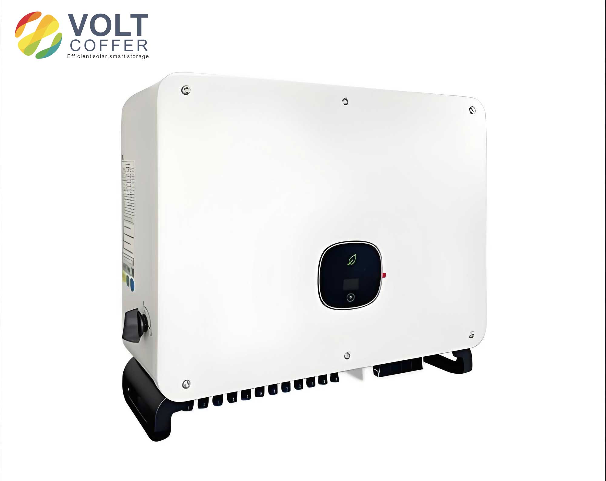
The power output from the combined PV and storage source, processed by the utility interactive inverter, is given by \( P_{inv} = P_{pv} + P_{es} \). The droop control laws for frequency (\(\omega\)) and voltage magnitude (\(E\)) are typically formulated as:
$$ \omega = \omega_0 – k_p (P – P_{set}) $$
$$ E = E_0 – k_q (Q – Q_{set}) $$
where \(\omega_0\) and \(E_0\) are the nominal frequency and voltage, \(k_p\) and \(k_q\) are the droop coefficients, \(P\) and \(Q\) are the measured output active and reactive power, and \(P_{set}\), \(Q_{set}\) are their setpoints. The power injection into the grid through an impedance \(X_s\) is:
$$ P = \frac{EV}{X_s} \sin\delta, \quad Q = \frac{EV}{X_s} \cos\delta – \frac{V^2}{X_s} $$
where \(V\) is the grid voltage magnitude and \(\delta\) is the power angle of the inverter voltage relative to the grid. Combining the droop laws, power flow equations, and the dynamics of the power calculation filter (with time constant related to \(\omega_c\)), leads to a set of nonlinear differential equations. A standard third-order dynamic model for the utility interactive inverter state vector \(\mathbf{x} = [\delta, \omega, E]^T\) can be expressed as:
$$ \dot{\delta} = \omega – \omega_0 $$
$$ \dot{\omega} = \omega_c (\omega_0 – \omega) – \omega_c k_p \left( \frac{EV}{X_s} \sin\delta – P_{set} \right) $$
$$ \dot{E} = \omega_c (E_0 – E) – \omega_c k_q \left( \frac{EV}{X_s} \cos\delta – \frac{V^2}{X_s} – Q_{set} \right) $$
This model captures the essential electromechanical transient behavior of the utility interactive inverter.
For stability analysis, especially of the large-signal or transient type, this third-order model, while useful, can be complex to handle directly. A powerful technique to simplify the analysis is the Singular Perturbation method. This method is ideal for systems with dynamics evolving at distinctly different speeds. In our utility interactive inverter model, the voltage magnitude \(E\) often has faster dynamics compared to the power angle \(\delta\) and frequency \(\omega\) dynamics, especially when the DC-link dynamics are stable. By defining a small perturbation parameter \(\epsilon\), we can separate the slow and fast states. The system is rewritten as:
$$ \dot{\mathbf{x}}_s = \mathbf{f}_s(\mathbf{x}_s, \mathbf{x}_f) $$
$$ \epsilon \dot{\mathbf{x}}_f = \mathbf{f}_f(\mathbf{x}_s, \mathbf{x}_f) $$
where \(\mathbf{x}_s = [\delta, \omega]^T\) are the slow states and \(\mathbf{x}_f = [E]\) is the fast state. The core idea is to solve for the quasi-steady-state of the fast dynamics (\(\mathbf{f}_f(\mathbf{x}_s, \mathbf{x}_f)=0\)) to obtain \(\mathbf{x}_f = \mathbf{h}(\mathbf{x}_s)\). Substituting this back into the slow dynamics yields a reduced-order model:
$$ \dot{\mathbf{x}}_s = \mathbf{f}_s(\mathbf{x}_s, \mathbf{h}(\mathbf{x}_s)) $$
This results in a second-order model primarily describing the angle/frequency dynamics, which is more amenable to analytical stability assessment methods like the equal area criterion or Lyapunov’s direct method.
To rigorously assess the transient stability region of the reduced-order utility interactive inverter model, Lyapunov’s direct method is employed. The goal is to construct a scalar energy-like function \(V(\mathbf{x})\) that is positive definite and has a negative definite time derivative along the trajectories of the system (\(\dot{V}(\mathbf{x}) < 0\)). Among various construction methods, the Variable Gradient Method offers significant flexibility for nonlinear systems. The procedure involves assuming a form for the gradient of \(V(\mathbf{x})\), denoted \(\nabla V\). For a second-order system with states \(z_1, z_2\) (representing deviations from equilibrium):
$$ \nabla V = \begin{bmatrix} a_{11}z_1 + a_{12}z_2 \\ a_{21}z_1 + a_{22}z_2 \end{bmatrix} $$
The coefficients \(a_{ij}\) are chosen to satisfy the curl condition (\(\frac{\partial}{\partial z_j}(\nabla V)_i = \frac{\partial}{\partial z_i}(\nabla V)_j\)) to ensure \(\nabla V\) is a valid gradient, and more importantly, to guarantee \(\dot{V} = (\nabla V)^T \dot{\mathbf{z}} < 0\). The Lyapunov function itself is then recovered by integration:
$$ V(\mathbf{z}) = \int_{0}^{\mathbf{z}} \nabla V \cdot d\mathbf{\zeta} $$
For our specific reduced-order utility interactive inverter model derived via singular perturbation, applying this method yields a function of the form:
$$ V(z_1, z_2) = \frac{1}{2} \alpha z_2^2 + \int_{0}^{z_1} \left( \beta \zeta – \gamma \sin(\zeta + \delta_0) + \eta \cos(\zeta + \delta_0) \right) d\zeta $$
where \(\alpha, \beta, \gamma, \eta\) are parameters depending on system and droop coefficients (\(k_p, k_q, X_s, etc.\)), and \(\delta_0\) is the equilibrium angle. The stability region can be estimated by the largest contour of this \(V(\mathbf{z})\) function inside which \(\dot{V} < 0\).
The integration of the energy storage system critically influences the parameters and equilibrium of the utility interactive inverter model. The ES provides an additional power source \(P_{es}\) that modifies the effective power setpoint or the initial power balance. This, in turn, affects the equilibrium point \((\delta_0, E_0)\) and the parameters within the Lyapunov function \(V(\mathbf{z})\). Consequently, the stability region in the state space changes. Typically, a properly sized and controlled ES can expand the region of attraction, allowing the system to recover from larger disturbances—a key benefit for system resilience. To quantify the performance and stability enhancements, a case study based on MATLAB/Simulink simulation is analyzed. The system parameters are summarized below:
| Component | Parameter | Value |
|---|---|---|
| Grid & Line | Voltage (L-L RMS) | 10 kV |
| Frequency | 50 Hz | |
| Equivalent Reactance \(X_s\) | 0.5 Ω | |
| Utility Interactive Inverter | Rated Power | 500 kVA |
| Droop Coefficients \(k_p, k_q\) | \(1 \times 10^{-4}\) | |
| Filter Cut-off Frequency \(\omega_c\) | 355 rad/s | |
| DC Link Voltage | 1500 V | |
| PV Array | Configuration | 50 series × 45 parallel |
| Open Circuit Voltage (\(V_{oc}\)) | 44.28 V per module | |
| Short Circuit Current (\(I_{sc}\)) | 8.56 A per module | |
| Battery Storage (BESS) | Capacity | 200 Ah @ 1500 V |
The simulation investigates three key aspects: power support, fluctuation suppression, and transient stability enhancement. First, under low solar irradiance (simulating 10% PV penetration), the utility interactive inverter output is compared with and without ES support. The ES successfully boosts the total active power injection \(P_{inv}\) to meet grid requirements, demonstrating its power support capability. Second, under rapidly changing irradiance, the output power fluctuation is analyzed. The performance metrics are compared in the following table:
| Operation Mode | Peak Time \(t_p\) (s) | Overshoot \(\sigma\) (%) | Settling Time \(t_s\) (s) |
|---|---|---|---|
| PV Only | 0.918 | 4.60 | 2.5 |
| PV with ES | 0.908 | 4.52 | 2.1 |
The integrated system shows reduced overshoot and faster settling, confirming the ES’s role in damping power oscillations managed by the utility interactive inverter. Third, for transient stability, a large disturbance (e.g., a step change in grid voltage or a fault) is simulated. The Lyapunov function \(V(\mathbf{z})\) constructed via the Variable Gradient Method is plotted for trajectories with and without ES. The critical energy level \(V_{cr}\) defining the stability boundary is found to be higher for the PV-ES system. This quantitatively translates to a larger permissible disturbance or a larger safety margin for the power angle \(\delta\). For illustration, the stability region projections can be compared based on the derived Lyapunov function parameters. A comparison of Lyapunov function construction methods for this inverter problem highlights the practicality of the Variable Gradient approach:
| Method | Applicability to Nonlinear Model | Complexity of Construction | |
|---|---|---|---|
| Krasovskii’s Method | Moderate | Low | Limited (often yields conservative, trivial regions) |
| Linear Matrix Inequality (LMI) | Requires linearization | High (computational) | Good for local analysis near equilibrium |
| Variable Gradient Method | High | Moderate (analytical) |
In conclusion, the stability analysis of a PV generation system integrated with energy storage is fundamentally linked to the dynamics of the interfacing utility interactive inverter. By employing a droop-control strategy, the inverter can provide vital grid-support functions. The high-order nonlinear model of this utility interactive inverter can be effectively reduced using the Singular Perturbation technique, simplifying the analysis. The application of the Variable Gradient Method to construct a Lyapunov function for the reduced-order model provides a powerful analytical tool to assess transient stability and quantify the stability region. Simulation studies confirm that the integrated energy storage system significantly enhances the performance of the overall system: it provides active power support during low PV generation, suppresses output power fluctuations, and, most importantly, increases the critical energy level and expands the power-angle stability region of the utility interactive inverter. This expanded stability margin is crucial for ensuring reliable operation under large disturbances in power systems with high penetration of renewable energy. Future work could focus on optimizing the droop coefficients and ES dispatch algorithms based on this stability region analysis to achieve coordinated control for multiple such inverters in a network.