
In recent years, the increasing demand for electrical energy and the rapid evolution of renewable green power sources have driven significant advancements in power electronics. Supported by technological innovations, societal needs, and government policies, solar energy has emerged as a pivotal resource in the power industry. The on-grid inverter serves as the critical electrical interface for integrating solar photovoltaic power generation into the grid. High-efficiency on-grid inverters ensure safe and reliable connections between renewable energy sources and the grid, facilitating easier adoption of新能源发电. Therefore, researching and improving control strategies to enhance the performance and quality of on-grid inverters is of paramount importance. Traditional control methods, such as proportional-integral (PI) control, often fall short in tracking sinusoidal signals without steady-state error and exhibit limited anti-interference capabilities in grid-connected applications, leading to reduced efficiency in photovoltaic systems. To address these issues, this study focuses on a control strategy based on the quasi-proportional resonant (QPR) controller. This approach improves upon proportional resonance control by incorporating a high-speed model predictive controller for three-phase reactive current and simultaneously handling harmonic disturbances, enabling the on-grid inverter to respond swiftly to grid variations. Through parameter design using variable methods and space vector pulse width modulation (SVPWM) for the inverter, we demonstrate the superiority of QPR control in eliminating steady-state error and resisting grid interference. In this article, I will delve into the structure, modeling, control strategies, parameter design, and simulation analysis of on-grid inverters, emphasizing the role of QPR control in optimizing performance.
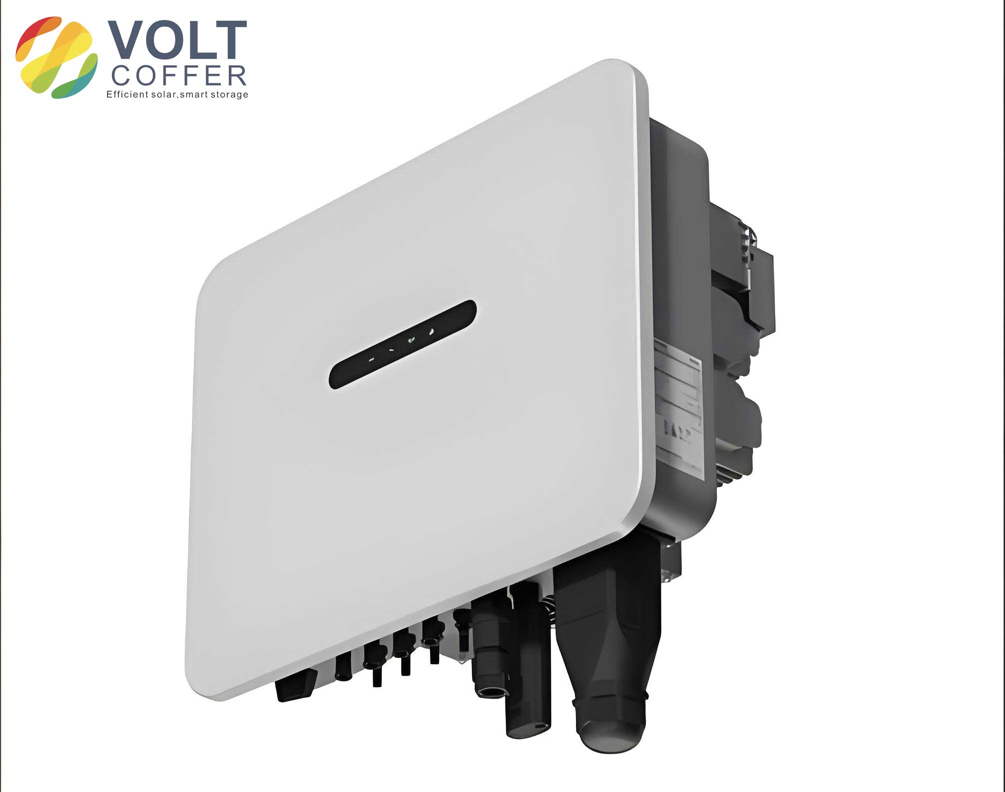
The on-grid inverter system typically comprises a full-bridge inverter circuit, filtering circuit, AC-side voltage preprocessing module, digital signal processor (DSP) control module, and an insulated gate bipolar transistor (IGBT) drive circuit. The output current passes through the inverter bridge and an inductor L before reaching the grid. During operation, the switching devices generate high-frequency harmonic currents due to their turning on and off, which the inductor filters to ensure the output current waveform aligns with the grid voltage in frequency and phase. When grid connection is initiated, the DSP detects the zero-crossing point of the grid voltage and triggers internal components to execute grid-connected control algorithms. It also performs phase-locking to track grid frequency variations, generating specific SVPWM control signals essential for inverter operation. These signals are then isolated through the IGBT bridge drive circuit to ensure reliable system performance. The core components of an on-grid inverter can be summarized in the following table:
| Component | Function | Key Characteristics |
|---|---|---|
| Full-Bridge Inverter | Converts DC to AC | Uses IGBT switches for high efficiency |
| Filter Inductor (L) | Filters harmonic currents | Reduces THD for smooth sinusoidal output |
| DSP Control Module | Executes control algorithms | Enables real-time processing and SVPWM generation |
| IGBT Drive Circuit | Isolates and amplifies control signals | Ensures safe switching of inverter bridges |
| Voltage Preprocessing | Conditions grid voltage signals | Facilitates accurate phase-locking and monitoring |
To develop an effective control strategy for the on-grid inverter, a precise mathematical model is essential. Assuming ideal conditions—such as symmetrical three-phase grid electromotive force, and ideal inductors, capacitors, resistors, and IGBT switches—we can derive the model using Kirchhoff’s laws. For the DC side, the relationship is given by:
$$ C \frac{du_{dc}}{dt} = i_{pv} – i_{dc} $$
$$ i_{dc} = i_a s_a + i_b s_b + i_c s_c $$
where \( C \) is the DC-link capacitance, \( u_{dc} \) is the DC voltage, \( i_{pv} \) is the photovoltaic current, \( i_{dc} \) is the inverter input current, and \( s_a, s_b, s_c \) are switching functions. For the AC side, applying Kirchhoff’s voltage law yields:
$$ \begin{bmatrix} u_a \\ u_b \\ u_c \end{bmatrix} = R \begin{bmatrix} i_a \\ i_b \\ i_c \end{bmatrix} + L \frac{d}{dt} \begin{bmatrix} i_a \\ i_b \\ i_c \end{bmatrix} + \begin{bmatrix} e_a \\ e_b \\ e_c \end{bmatrix} $$
Here, \( u_a, u_b, u_c \) are the inverter output voltages, \( i_a, i_b, i_c \) are the grid currents, \( R \) and \( L \) are the filter resistance and inductance, and \( e_a, e_b, e_c \) are the grid voltages. To simplify analysis, we transform this model from the abc stationary coordinate system to the αβ coordinate system using the Clarke transformation matrix:
$$ T_{abc/\alpha\beta} = \frac{2}{3} \begin{bmatrix} 1 & -\frac{1}{2} & -\frac{1}{2} \\ 0 & \frac{\sqrt{3}}{2} & -\frac{\sqrt{3}}{2} \end{bmatrix} $$
Applying this transformation, we obtain the model in αβ coordinates:
$$ L \frac{d}{dt} \begin{bmatrix} i_\alpha \\ i_\beta \end{bmatrix} = -R \begin{bmatrix} i_\alpha \\ i_\beta \end{bmatrix} – \begin{bmatrix} u_\alpha \\ u_\beta \end{bmatrix} – \begin{bmatrix} e_\alpha \\ e_\beta \end{bmatrix} $$
This representation reveals that in the αβ frame, the input currents are decoupled, with \( i_\alpha \) and \( i_\beta \) independent of each other, simplifying control design. For comparison, the Park transformation can further convert the model to the dq rotating coordinate system:
$$ T_{\alpha\beta/dq} = \begin{bmatrix} \cos \omega t & \sin \omega t \\ -\sin \omega t & \cos \omega t \end{bmatrix} $$
leading to:
$$ L \frac{d}{dt} \begin{bmatrix} i_d \\ i_q \end{bmatrix} = \begin{bmatrix} -R & \omega L \\ -\omega L & -R \end{bmatrix} \begin{bmatrix} i_d \\ i_q \end{bmatrix} – \frac{u_{dc}}{2} \begin{bmatrix} u_d \\ u_q \end{bmatrix} – \begin{bmatrix} e_d \\ e_q \end{bmatrix} $$
where \( \omega \) is the grid angular frequency. The dq model introduces cross-coupling terms (\( \omega L \)), necessitating decoupling control in traditional PI-based strategies. However, the αβ model avoids this complexity, making it advantageous for resonant control methods. The mathematical models highlight key parameters that influence on-grid inverter behavior, as summarized below:
| Parameter | Symbol | Role in Model |
|---|---|---|
| Filter Inductance | \( L \) | Determines current ripple and harmonic filtering |
| Filter Resistance | \( R \) | Affects power losses and damping characteristics |
| DC-Link Capacitance | \( C \) | Stabilizes DC voltage and reduces ripple |
| Grid Frequency | \( \omega \) | Influences transformation and control dynamics |
| Switching Functions | \( s_a, s_b, s_c \) | Represent inverter switching states for modulation |
Control strategies for on-grid inverters are crucial for achieving high-performance grid integration. Traditional methods include hysteresis comparison control, current predictive control, deadbeat control, repetitive control, and PI control. Hysteresis control is simple and offers good dynamic performance, but its variable switching frequency complicates filter design and increases harmonic content. Current predictive control relies on accurate mathematical models, making it sensitive to parameter variations. Deadbeat control provides fast dynamic response and high tracking accuracy but requires heavy computation and lacks robustness. Repetitive control, based on periodic signal theory, achieves minimal steady-state error for periodic signals but suffers from poor dynamic performance. PI control can eliminate DC bias but requires coordinate transformations (Clarke and Park) for decoupling in rotating frames, adding complexity. To overcome these limitations, proportional resonant (PR) control has been proposed. PR control operates in the stationary coordinate system, eliminating the need for rotational transformations and enabling zero steady-state error for sinusoidal tracking. The ideal PR controller transfer function is:
$$ G_{PR}(s) = K_P + \frac{2K_r s}{s^2 + \omega_n^2} $$
where \( K_P \) is the proportional gain, \( K_r \) is the resonant gain, and \( \omega_n \) is the resonant frequency (typically the grid fundamental frequency). At \( \omega_n \), the gain approaches infinity, allowing perfect tracking of sinusoidal references. However, ideal PR controllers are challenging to implement due to infinite gain and limited bandwidth, which reduces robustness to grid frequency variations. Therefore, the quasi-proportional resonant (QPR) controller is introduced, featuring a modified transfer function:
$$ G_{QPR}(s) = K_P + \frac{2K_r \omega_c s}{s^2 + 2\omega_c s + \omega_n^2} $$
Here, \( \omega_c \) is the cutoff frequency, which broadens the bandwidth and improves adaptability to grid frequency shifts. The QPR controller maintains high gain near \( \omega_n \) without being infinite, reducing sensitivity while enhancing anti-interference capabilities. This makes it particularly suitable for on-grid inverters facing harmonic disturbances and voltage imbalances. The advantages of QPR control over other methods can be summarized as follows:
| Control Method | Strengths | Weaknesses | Suitability for On-Grid Inverters |
|---|---|---|---|
| Hysteresis Control | Simple, fast dynamic response | Variable switching frequency, high harmonics | Low for grid-tied due to harmonic issues |
| Predictive Control | High accuracy with precise models | Sensitive to parameter changes | Moderate, requires robust modeling |
| Deadbeat Control | Rapid tracking, minimal delay | Computationally intensive, poor robustness | Limited for real-time applications |
| Repetitive Control | Zero steady-state error for periodic signals | Slow dynamic response | Good for steady-state but not transient |
| PI Control | Effective for DC signals, widely used | Needs decoupling, poor for AC tracking | Moderate with complex transformations |
| PR Control | Zero error for sinusoidal signals, no transformation needed | Infinite gain impractical, narrow bandwidth | High if bandwidth limitations addressed |
| QPR Control | Zero error, broad bandwidth, robust to frequency shifts | Parameter tuning required | Excellent for grid-connected applications |
The design of QPR controller parameters—\( K_P \), \( K_r \), and \( \omega_c \)—is critical for optimal performance. By analyzing the frequency response, we can understand how each parameter affects the system. First, setting \( K_P = 0 \) and \( \omega_c = 1 \), variations in \( K_r \) show that \( K_r \) directly influences the gain at the resonant frequency but does not affect bandwidth. Increasing \( K_r \) reduces steady-state error but may amplify harmonics if too high, degrading grid current quality. Second, with \( K_P = 0 \) and \( K_r = 1 \), changes in \( \omega_c \) demonstrate that \( \omega_c \) impacts both bandwidth and gain: a larger \( \omega_c \) widens the bandwidth and increases gain at non-fundamental frequencies, enhancing adaptability to grid frequency fluctuations. Third, fixing \( \omega_c = 3.14 \, \text{rad/s} \) and \( K_r = 100 \), adjusting \( K_P \) reveals that \( K_P \) affects harmonic impedance without altering gain or bandwidth; higher \( K_P \) improves anti-interference ability but can cause instability if excessive. Therefore, parameter design should follow a systematic approach: select \( \omega_c \) based on desired bandwidth, choose \( K_r \) to achieve sufficient gain at the fundamental frequency, and determine \( K_P \) to balance harmonic impedance and stability, considering interactions between parameters. The effects of these parameters are quantified below:
| Parameter | Effect on Gain | Effect on Bandwidth | Practical Design Guideline |
|---|---|---|---|
| \( K_P \) | No direct effect | No effect | Increase for higher harmonic impedance, but keep moderate to avoid oscillation |
| \( K_r \) | Directly proportional to gain at \( \omega_n \) | Negligible effect | Choose to ensure high gain at fundamental frequency, typically 50-200 |
| \( \omega_c \) | Increases gain at non-fundamental frequencies | Directly proportional to bandwidth | Set based on expected grid frequency variations, e.g., 5-10 rad/s |
To validate the QPR control strategy for on-grid inverters, simulation analysis was conducted using Matlab/Simulink. The system parameters were set as follows: grid voltage RMS of 380 V, filter inductance of 10 mH, DC source voltage of 800 V, and QPR controller parameters \( K_P = 40 \), \( K_r = 100 \), \( \omega_c = 5 \, \text{rad/s} \). The simulation included modules for phase-locked loop (PLL), SVPWM, and the QPR-controlled inverter. The PLL module effectively tracked grid phase, with transformed voltages \( V_d \) and \( V_q \) showing stable waveforms and a locked phase周期 of 0.02 s. The SVPWM module generated switching signals with a saddle-shaped modulation wave, improving DC voltage utilization and harmonic suppression. For the on-grid inverter, the QPR controller demonstrated excellent performance: the actual grid current closely tracked the reference sinusoidal current with negligible steady-state error, achieving precise tracking within 0.002 seconds. In comparison, traditional PI control exhibited noticeable steady-state error and slower response, while improved PI control showed some enhancement but still lagged behind QPR control. Harmonic analysis revealed that QPR control achieved a total harmonic distortion (THD) of 1.63%,优于改进PI控制的THD of 1.71% reported in literature, highlighting its superior harmonic suppression. The simulation results underscore the effectiveness of QPR control in enhancing on-grid inverter performance. Key simulation outcomes are summarized below:
| Performance Metric | QPR Control | Traditional PI Control | Improved PI Control |
|---|---|---|---|
| Steady-State Error | Nearly zero | Significant | Reduced but present |
| Tracking Speed | Within 0.002 s | Slower, over 0.005 s | Moderate, around 0.003 s |
| THD of Grid Current | 1.63% | Typically above 2% | 1.71% (as per literature) |
| Robustness to Grid Variations | High due to broad bandwidth | Low, sensitive to frequency shifts | Moderate with tuning |
| Implementation Complexity | Low, no coordinate transformations needed | High, requires decoupling and transformations | Moderate, may need additional compensation |
The mathematical foundation of QPR control can be further explored through frequency response analysis. The magnitude and phase of the QPR transfer function are given by:
$$ |G_{QPR}(j\omega)| = \sqrt{ \left( K_P + \frac{2K_r \omega_c \omega^2}{(\omega_n^2 – \omega^2)^2 + (2\omega_c \omega)^2} \right)^2 } $$
$$ \angle G_{QPR}(j\omega) = \tan^{-1}\left( \frac{2K_r \omega_c \omega}{K_P(\omega_n^2 – \omega^2) + 2K_r \omega_c \omega^2} \right) $$
These equations help in tuning parameters for desired gain margins and phase margins. Additionally, the closed-loop transfer function of the on-grid inverter with QPR control can be derived from the αβ model. Assuming a current control loop with feedback gain \( H_I \) and PWM gain \( K_{PWM} \), the output current \( i_\alpha \) in response to reference \( i_\alpha^* \) and grid voltage disturbance \( e_\alpha \) is:
$$ i_\alpha = \frac{K_{PWM} G_{QPR}(s)}{H_I (sL + R)(T_s s + 1) + K_{PWM} G_{QPR}(s)} i_\alpha^* – \frac{1}{H_I (sL + R)(T_s s + 1) + K_{PWM} G_{QPR}(s)} e_\alpha $$
where \( T_s \) is the sampling time. At the resonant frequency \( \omega_n \), \( G_{QPR}(j\omega_n) \) is large, making the first term approach \( i_\alpha^* \) and the second term negligible, thus achieving disturbance rejection. This formulation underscores the importance of QPR control in mitigating grid voltage impacts on on-grid inverter output.
In practical applications, on-grid inverters must comply with grid codes requiring low THD (e.g., below 5%) and fast response to grid changes. QPR control facilitates this by offering adjustable bandwidth and high gain at selected frequencies. For instance, to suppress specific harmonics like the 5th or 7th, multiple resonant controllers can be paralleled at respective frequencies, enhancing harmonic immunity. The overall control structure for a three-phase on-grid inverter with QPR control involves measuring grid voltages and currents, transforming them to αβ coordinates, comparing with references, processing through QPR controllers, and generating SVPWM signals. This structure eliminates the need for Park transformations, reducing computational burden and potential errors. Moreover, the integration of model predictive control for reactive current handling further boosts dynamic performance, as mentioned earlier. The synergy between QPR and predictive elements enables robust operation under varying grid conditions, such as voltage sags or frequency deviations.
Looking ahead, advancements in digital signal processing and power electronics will continue to refine on-grid inverter control. Techniques like adaptive QPR control, where parameters adjust in real-time based on grid conditions, could offer even greater resilience. Additionally, the proliferation of distributed generation systems underscores the need for inverters that not only inject power but also provide grid-support functions like voltage regulation and frequency stabilization. QPR-based strategies, with their inherent flexibility and accuracy, are well-positioned to meet these demands. Simulation studies, as presented, provide a foundation for hardware implementation, though practical considerations like noise, component tolerances, and thermal effects must be addressed. Field tests and prototype developments would further validate the efficacy of QPR control in real-world on-grid inverter applications.
In conclusion, the quasi-proportional resonant control strategy represents a significant improvement for on-grid inverters, addressing the limitations of traditional PI control and other methods. By operating in the stationary coordinate system, QPR control achieves zero steady-state error in tracking sinusoidal currents, enhances anti-interference capabilities, and simplifies implementation. Through careful parameter design and simulation验证, we have demonstrated its superiority in terms of tracking precision, harmonic suppression, and response speed. As renewable energy integration becomes increasingly critical, optimizing on-grid inverter performance through advanced control strategies like QPR will play a vital role in ensuring grid stability and efficiency. Future work may explore hybrid approaches combining QPR with other techniques for even broader operational robustness.