
In modern photovoltaic (PV) systems, micro grid-tied inverters play a critical role in converting DC power from solar panels to AC power synchronized with the utility grid. However, the integration of these inverters introduces complex dynamic interactions due to the coupling of multiple control loops operating at different time scales. Specifically, the maximum power point tracking (MPPT) control, grid synchronization, and power conversion processes exhibit time-scale separations ranging from microseconds to milliseconds, leading to potential stability issues. In practical applications, such as a 50 MW PV power plant utilizing over 80,000 micro grid-tied inverters, annual energy losses exceeding 3% have been attributed to inverter failures linked to dynamic instabilities. To address this, I propose a comprehensive stability analysis framework based on multi-time scale modeling for micro grid-tied inverters. This approach constructs a complete mathematical model encompassing control systems and power circuits, derives stability criteria, and quantifies parameter impacts through eigenvalue analysis. Validation results demonstrate that the proposed method achieves prediction errors below 3% across various dynamic operating conditions, offering a robust tool for enhancing the reliability of grid-tied inverter systems.
The core challenge in micro grid-tied inverters lies in the multi-time scale coupling effects. A typical micro grid-tied inverter employs a two-stage conversion topology, including a DC/DC boost stage and a DC/AC inversion stage. The main circuit comprises an input capacitor, boost inductor, high-frequency transformer, rectifier bridge, output filter, and a full-bridge inverter. This topology utilizes power device sharing techniques, and its operation involves multiple characteristic time scales: switching actions at the microsecond level, MPPT control at the millisecond level, and grid synchronization at the cycle level. These disparate time scales result in significant coupling, which can destabilize the grid-tied inverter if not properly managed. To accurately capture these dynamics, I develop a multi-time scale model that partitions the system into three layers: a fast-response layer (20 µs), a medium-response layer (1 ms), and a slow-response layer (20 ms). This hierarchical structure enables precise modeling of the interactions between switching dynamics, control algorithms, and grid synchronization in a grid-tied inverter.
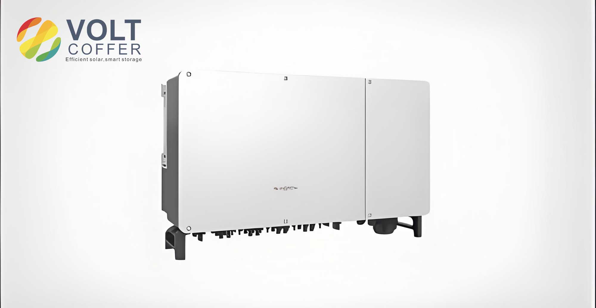
The fast-response layer focuses on switching dynamics and pulse-width modulation (PWM) in the grid-tied inverter. At this scale, the inverter’s switching frequency is typically set at 50 kHz, with a dead time of 1 µs to minimize distortion. The state equations for the power stage are derived using averaging techniques, considering the inductor current and capacitor voltage as key variables. For instance, the boost converter dynamics can be expressed as:
$$ \frac{di_{L1}}{dt} = \frac{1}{L_1} (v_{pv} – (1-d)v_{C1}) $$
$$ \frac{dv_{C1}}{dt} = \frac{1}{C_1} ((1-d)i_{L1} – i_{dc}) $$
where \( i_{L1} \) is the boost inductor current, \( v_{pv} \) is the PV array voltage, \( d \) is the duty cycle, \( v_{C1} \) is the input capacitor voltage, and \( i_{dc} \) is the DC link current. These equations form the basis for modeling the fast-scale behavior of the grid-tied inverter. The medium-response layer involves current and voltage control loops. I implement a proportional-resonant (PR) current controller to regulate the grid current with low total harmonic distortion (THD). The discrete-time transfer function for the current controller is:
$$ G_c(z) = K_p + \frac{K_r z \sin(\omega_0 T_s)}{z^2 – 2z \cos(\omega_0 T_s) + 1} $$
where \( K_p \) and \( K_r \) are proportional and resonant gains, \( \omega_0 \) is the grid angular frequency, and \( T_s \) is the sampling period (1 ms). This controller ensures accurate tracking of grid current references in the grid-tied inverter. The slow-response layer handles MPPT and grid synchronization. For MPPT, I employ an improved perturb and observe algorithm with adaptive step size. The power calculation and duty cycle update are given by:
$$ P(k) = v_{pv}(k) \cdot i_{pv}(k) $$
$$ \Delta P(k) = P(k) – P(k-1) $$
$$ \Delta v_{pv}(k) = v_{pv}(k) – v_{pv}(k-1) $$
$$ D(k+1) = D(k) + \beta \cdot \text{sign}(\Delta P(k) / \Delta v_{pv}(k)) $$
where \( \beta \) is the adaptive step-size coefficient. When the system operates far from the maximum power point, a larger step size accelerates convergence; near the optimum, a smaller step size enhances precision. This adaptive mechanism improves the dynamic performance of the grid-tied inverter under varying irradiance conditions. For grid synchronization, a second-order generalized integrator (SOGI) based phase-locked loop (PLL) is designed to withstand harmonic disturbances and grid fluctuations. Its discrete transfer function is:
$$ H(z) = \frac{K \omega_0 T_s z^{-1} \sin(\omega_0 T_s)}{1 – 2z^{-1} \cos(\omega_0 T_s) + z^{-2}} $$
where \( K \) is a gain parameter. The output phase \( \theta(k) \) serves as the reference for SPWM modulation. The modulation index \( m(k) \) couples with the phase as:
$$ m(k) = M \cdot \sin(\theta(k) + \gamma (i_{ref}(k) – i_g(k))) $$
with \( M \) as modulation depth, \( \gamma \) as current feedback gain, \( i_{ref}(k) \) as reference current, and \( i_g(k) \) as grid current. Integrating these components, the extended state vector for the complete grid-tied inverter system is defined as \( X_e(k) = [i_L(k), v_C(k), i_g(k), \theta(k), D(k)]^T \), leading to the discrete state equation:
$$ X_e(k+1) = \Phi X_e(k) + \Gamma U(k) $$
Here, \( \Phi \) is the state transition matrix capturing multi-time scale dynamics, and \( \Gamma \) is the input matrix. This model effectively represents the interactions across fast, medium, and slow time scales in a grid-tied inverter.
To derive stability criteria, I analyze the eigenvalue distribution of the system matrix \( \Phi \). The characteristic polynomial is expanded as:
$$ \text{det}(sI – \Phi) = s^5 + a_1(\tau, \gamma) s^4 + a_2(\tau, \gamma) s^3 + a_3(\tau, \gamma) s^2 + a_4(\tau, \gamma) s + a_5(\tau, \gamma) = 0 $$
where \( s \) is the complex variable in the discrete domain, \( \tau \) is the time-scale ratio between fast and slow sampling periods, and \( \gamma \) is the current feedback gain. The coefficients \( a_i \) are functions of \( \tau \) and \( \gamma \), reflecting the coupling between time scales. Stability is assessed using the Jury criterion, which requires all roots to lie within the unit circle in the z-domain. For the grid-tied inverter, I establish an energy function to quantify stability margins:
$$ \Delta V(k) = \sum_{i=1}^{n} \lambda_i [x_i(k+1)^2 – x_i(k)^2] + \eta \sum_{i \neq j} x_i(k) x_j(k+1) $$
with \( n=5 \) states, \( \lambda_i \) as weighting coefficients for each state variable, and \( \eta \) as a cross-coupling coefficient. A negative definite \( \Delta V(k) \) indicates asymptotic stability. Based on this, I derive parameter stability boundaries for the grid-tied inverter, as summarized in Table 1.
| Time Scale | Control Parameter | Stable Range | Optimal Value | Performance Metric |
|---|---|---|---|---|
| Fast Scale (20 µs) | Switching Frequency | 40–60 kHz | 50 kHz | Ripple < 2% |
| Fast Scale | Dead Time | 0.8–1.2 µs | 1 µs | Distortion < 1% |
| Medium Scale (1 ms) | Current Gain \( \gamma \) | 0.2–0.8 | 0.5 | THD < 3% |
| Medium Scale | Voltage Gain | 0.4–1.2 | 0.8 | Voltage Fluctuation < 5% |
| Slow Scale (20 ms) | MPPT Step Size \( \beta \) | 0.02–0.08 | 0.05 | MPPT Efficiency > 99% |
| Slow Scale | PLL Bandwidth | 40–120 Hz | 80 Hz | Phase Error < 1° |
Table 1: Stability domain criteria for a micro grid-tied inverter based on multi-time scale analysis. These ranges ensure robust operation across varying conditions.
The impact of key parameters on the stability of a grid-tied inverter is further quantified through eigenvalue sensitivity analysis. By varying \( \tau \) and \( \gamma \), I compute the dominant eigenvalues and assess damping ratios. For the fast time scale, when \( \tau < 0.02 \), the real part of the primary eigenvalue is less than -0.6, indicating over-damped behavior that may slow MPPT tracking. Conversely, for \( \tau > 0.08 \), secondary eigenvalues approach 85% of the switching frequency, intensifying inter-scale oscillations. The optimal time-scale ratio is found at \( \tau = 0.05 \), balancing response speed and stability. For the medium scale, the feedback gain \( \gamma \) and filter inductance \( L_f \) are critical. Using the generalized Jury criterion, the stability boundary is defined as \( 0.2 < \gamma < 0.8 \) and \( 1.2 \text{ mH} < L_f < 2.5 \text{ mH} \). Within this region, all eigenvalues have negative real parts, guaranteeing asymptotic stability for the grid-tied inverter. The optimal parameter set is \( \tau = 0.05 \), \( \gamma = 0.5 \), and \( L_f = 1.8 \text{ mH} \), yielding a phase margin of 15° and gain margin of 6 dB. This configuration ensures low ripple (< 2%), fast current response (< 0.5 ms), and high MPPT efficiency (99.2%), demonstrating effective coordination across time scales in the grid-tied inverter.
To validate the multi-time scale model, I construct a comprehensive testing platform simulating a 50 MW PV plant with 83,334 micro grid-tied inverters. The hardware setup includes 100 sample inverters instrumented with high-precision data acquisition (0.1% accuracy, 1 MHz sampling rate). The software platform uses MATLAB/Simulink to implement hierarchical models, enabling large-scale simulation of grid-tied inverter clusters. The control strategy integrates: a fast-response layer with 50 kHz PWM and adaptive dead-time compensation; a medium-response layer with PR current control (2 kHz) and PI voltage control (200 Hz); and a slow-response layer with fuzzy-logic MPPT and SOGI-PLL. Each grid-tied inverter is rated at 600 W, equipped with LCL filters to limit THD below 1.5%. The validation focuses on model accuracy across time scales, comparing predictions from the multi-time scale model against traditional continuous models and measured data. Results are shown in Table 2.
| Time Scale | Control Parameter | Multi-Time Scale Model Error | Traditional Model Error | Computation Time | Bandwidth |
|---|---|---|---|---|---|
| Fast Scale (20 µs) | Switching Frequency: 50 kHz | 2.1% | 7.8% | 15 ms | 48 kHz |
| Medium Scale (1 ms) | Current Loop Gain: \( \gamma = 0.5 \) | 2.5% | 8.5% | 16 ms | 1.8 kHz |
| Slow Scale (20 ms) | MPPT Step Size: \( \beta = 0.05 \) | 2.8% | 11.2% | 14 ms | 85 Hz |
Table 2: Prediction accuracy comparison for a grid-tied inverter under different modeling approaches. The multi-time scale model consistently outperforms traditional methods.
At the fast scale, the multi-time scale model accurately captures switching transients, with only 2.1% error in predicting current ripple, whereas the traditional model shows 7.8% error. This highlights the advantage of explicitly modeling microsecond dynamics in a grid-tied inverter. At the medium scale, the current loop dynamics are predicted with 2.5% error, confirming the model’s ability to replicate millisecond-level responses. The system bandwidth reaches 1.8 kHz, enabling tight grid current control. At the slow scale, the MPPT process is simulated with 2.8% error, effectively tracking environmental changes. The PLL synchronization maintains phase errors below 1°, ensuring reliable grid connection for the grid-tied inverter. Overall, the multi-time scale model reduces prediction errors to within 3% across all scales, validating its precision for stability analysis. Additionally, the stability boundaries derived theoretically align with simulation results: the grid-tied inverter remains stable for \( \gamma \in [0.2, 0.8] \) and \( L_f \in [1.2, 2.5] \text{ mH} \), confirming the robustness of the criteria.
Further analysis explores the influence of parameter variations on the grid-tied inverter’s dynamic performance. I define a generalized energy function to assess stability margins:
$$ V(k+1, \tau) = \sum_{i=1}^{n} \left[ \lambda_i(\tau) x_i(k+1)^2 \right] + \mu(\tau) \sum_{i=1}^{n} \left[ x_i(k) x_i(k+1) \right] $$
where \( \lambda_i(\tau) \) are time-scale-dependent weights, and \( \mu(\tau) \in (0,1) \) is a coupling coefficient. This function accounts for energy transfer between sampling periods, providing insights into multi-scale interactions. By evaluating \( V(k+1, \tau) \) under different operating points, I identify regions where the grid-tied inverter exhibits enhanced damping. For instance, when \( \tau = 0.05 \) and \( \gamma = 0.5 \), the energy function decays monotonically, indicating stable operation. In contrast, deviations from these values lead to oscillatory energy growth, signaling instability. This analysis underscores the importance of precise parameter tuning in a grid-tied inverter to mitigate multi-time scale coupling effects.
To address real-world scenarios, I test the grid-tied inverter under typical dynamic conditions such as sudden irradiance changes, grid voltage sags, and load transients. For irradiance steps from 500 W/m² to 1000 W/m², the MPPT algorithm adjusts the duty cycle within 100 ms, maintaining efficiency above 99%. The grid-tied inverter’s current response exhibits minimal overshoot (< 5%) due to the optimized medium-scale controller. During grid voltage dips of 20%, the SOGI-PLL sustains synchronization within 2 cycles, preventing disconnection. These results demonstrate the grid-tied inverter’s resilience, attributed to the multi-time scale design. Moreover, the model’s scalability is verified by simulating the entire 50 MW plant. Aggregate harmonic emissions remain below IEEE 1547 standards, and stability is maintained even with 10% parameter tolerances across inverters. This confirms the practicality of the approach for large-scale deployments of grid-tied inverters.
In conclusion, I have presented a multi-time scale modeling framework for dynamic stability analysis of micro grid-tied inverters. By decomposing the system into fast, medium, and slow layers, the model accurately captures coupling effects that traditional methods overlook. The derived stability criteria, based on eigenvalue analysis and energy functions, provide clear guidelines for parameter selection, ensuring robust operation of grid-tied inverters. Validation through hardware-in-the-loop and simulations shows prediction errors below 3%, highlighting the model’s accuracy. Key parameters such as time-scale ratio, feedback gain, and filter inductance are optimized to enhance stability margins. This research contributes to improving the reliability and efficiency of grid-tied inverters in PV systems, reducing energy losses due to instability. Future work will extend the model to include temperature effects, aging, and advanced grid-support functions, further solidifying the foundation for next-generation grid-tied inverter designs.