
In recent years, the integration of solar energy systems with agricultural practices has gained significant attention as a sustainable solution to address energy demands while maintaining food production. As a researcher focused on renewable energy applications, I have explored the shading effects induced by photovoltaic panels in agrivoltaic systems. The primary objective of this study is to analyze how varying configurations of solar panels influence shading distribution and solar radiation intensity beneath the arrays, using advanced simulation tools like Ladybug. This investigation is crucial for optimizing photovoltaic agricultural setups to ensure adequate light conditions for crop growth while maximizing energy generation.
Agrivoltaics, which combines photovoltaic energy production with agricultural activities, presents a promising approach to land-use efficiency. However, the shading caused by solar panels can significantly alter the microclimate underneath, affecting plant photosynthesis and yield. Through this research, I aim to provide insights into the dynamics of shading effects, considering parameters such as panel spacing, installation height, and tilt angle. By employing three-dimensional simulation techniques, I have modeled various scenarios to quantify shading rates and cumulative solar irradiation, which are critical for designing efficient agrivoltaic systems.
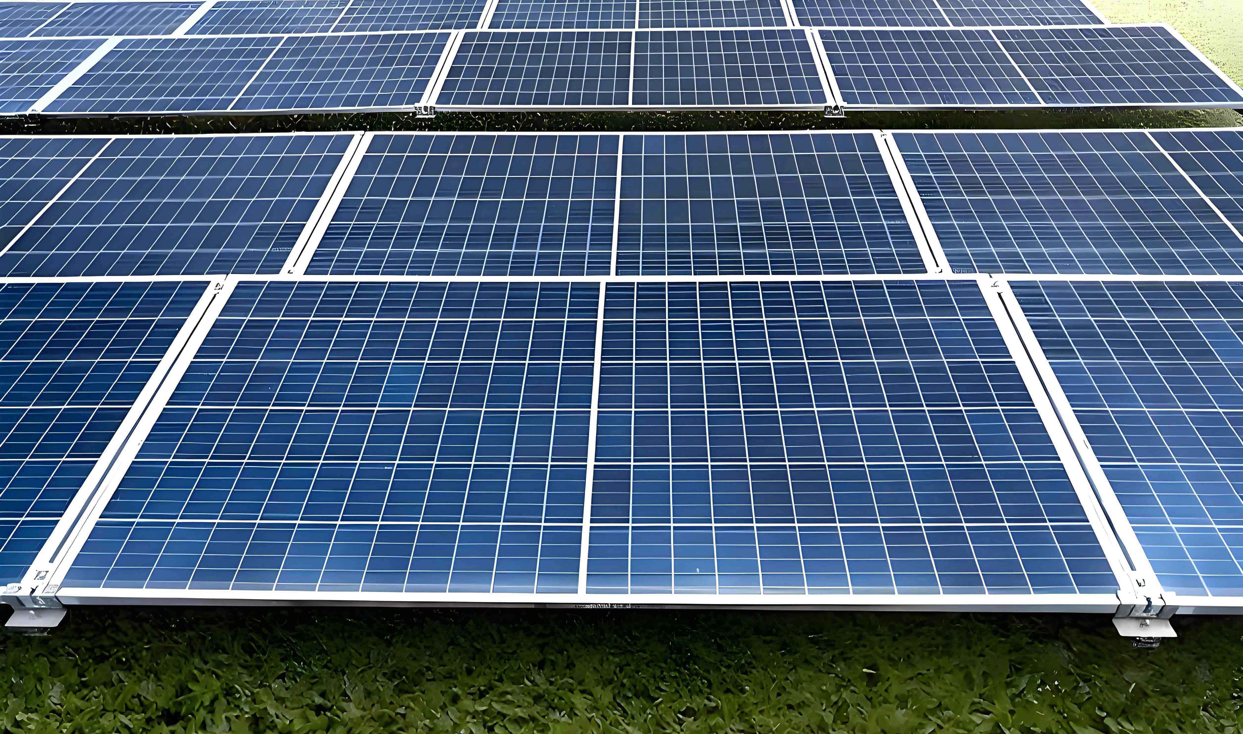
The methodology of this study revolves around the use of Ladybug, a powerful plugin for environmental analysis in building information modeling. I developed detailed 3D models of photovoltaic arrays and simulated solar radiation patterns based on meteorological data from two distinct locations with varying solar characteristics. These locations were selected to represent different climatic conditions, enabling a comprehensive analysis of shading effects. The key variables investigated include the spacing between panels along the x-axis (20 cm, 50 cm, and 100 cm), installation height (150 cm, 200 cm, and 250 cm), and tilt angle (0°, 15°, and 30°). The y-axis spacing was fixed at 50 cm to maintain consistency across simulations. All analyses were conducted for the summer solstice (June 21) during peak solar hours from 9:00 to 16:00, as this period represents the highest solar radiation intensity, which is critical for assessing shading impacts.
To accurately capture the shading effects, I divided the area beneath the photovoltaic arrays into a grid of 1 m × 1 m cells. This allowed for a granular analysis of cumulative irradiance and shading rates across different regions under the panels. The solar radiation data were processed using Ladybug’s solar radiation analysis module, which calculates direct and diffuse radiation based on sun path and weather files. The shading rate (S) for each grid cell was derived using the formula: $$ S = \left(1 – \frac{I_{\text{shaded}}}{I_{\text{open}}}\right) \times 100\% $$ where \( I_{\text{shaded}} \) is the cumulative irradiance in the shaded area and \( I_{\text{open}} \) is the cumulative irradiance in an open area without obstruction. This formula helps quantify the percentage reduction in solar radiation due to photovoltaic panel shading.
The simulation results revealed significant variations in shading rates based on the configuration of the photovoltaic arrays. For instance, when examining the effect of panel spacing, I observed that increasing the x-axis spacing from 20 cm to 100 cm led to a substantial decrease in shading rates. This is because wider spacing allows more direct sunlight to penetrate the underlying area, reducing the extent of shadow coverage. The relationship between spacing and shading rate can be expressed using a linear approximation: $$ S = a – b \cdot d $$ where \( S \) is the shading rate, \( d \) is the spacing in cm, and \( a \) and \( b \) are constants derived from regression analysis of the simulation data. This equation highlights the inverse correlation between panel spacing and shading intensity, which is vital for designing photovoltaic systems that balance energy production and agricultural needs.
In terms of installation height, the simulations showed that higher placements of solar panels (e.g., 250 cm) resulted in increased shading rates in certain regions beneath the arrays. This phenomenon occurs because elevated panels cast longer shadows during peak sun hours, especially when the sun is at lower angles. However, the distribution of shading is not uniform; areas directly under the panels experience higher shading rates, while edges receive more sunlight. The cumulative irradiance under different heights can be modeled using the formula: $$ I_{\text{cum}} = I_0 \cdot e^{-k \cdot h} $$ where \( I_{\text{cum}} \) is the cumulative irradiance, \( I_0 \) is the irradiance in open areas, \( h \) is the installation height, and \( k \) is an attenuation coefficient specific to the panel configuration. This exponential decay model underscores the trade-off between panel height and light availability for crops.
The tilt angle of photovoltaic panels also played a critical role in modulating shading effects. As the tilt angle increased from 0° to 30°, the shading rate decreased due to changes in the angle of incidence of solar rays. This adjustment allows more sunlight to reach the ground, particularly during periods of high solar altitude. The effect of tilt angle on shading rate can be described by: $$ S = S_0 – c \cdot \theta $$ where \( S_0 \) is the shading rate at 0° tilt, \( \theta \) is the tilt angle in degrees, and \( c \) is a constant that depends on geographic and temporal factors. This linear relationship emphasizes the importance of optimizing tilt angles to minimize shading while maintaining efficient energy capture by the photovoltaic panels.
To summarize the findings, I have compiled several tables that illustrate the variations in shading rates and cumulative irradiance under different photovoltaic panel configurations. These tables provide a quantitative basis for comparing the impacts of spacing, height, and tilt angle on agrivoltaic systems.
| Spacing (cm) | Location A Max Shading Rate | Location A Min Shading Rate | Location B Max Shading Rate | Location B Min Shading Rate |
|---|---|---|---|---|
| 20 | 65.1 | 41.7 | 64.4 | 50.5 |
| 50 | 56.3 | 36.0 | 58.5 | 45.8 |
| 100 | 44.0 | 36.6 | 44.8 | 40.9 |
Table 1 demonstrates that as the spacing between photovoltaic panels increases, both maximum and minimum shading rates decrease. This trend is consistent across both locations, indicating that wider spacing enhances light penetration and reduces shadowing effects. For example, at 100 cm spacing, the maximum shading rate drops to approximately 44% in both locations, compared to over 64% at 20 cm spacing. This reduction is critical for crops that require sufficient sunlight for photosynthesis, as it minimizes the risk of light deprivation.
| Height (cm) | Location A Cumulative Irradiance | Location B Cumulative Irradiance | Average Shading Rate (%) |
|---|---|---|---|
| 150 | 0.57 – 0.95 | 1.28 – 1.78 | 60.5 |
| 200 | 0.50 – 0.97 | 1.08 – 1.60 | 65.0 |
| 250 | 0.54 – 1.12 | 1.02 – 1.98 | 68.5 |
Table 2 highlights the impact of installation height on cumulative irradiance and shading rates. Higher installations generally lead to lower cumulative irradiance values in the shaded regions, resulting in higher average shading rates. For instance, at 250 cm height, the average shading rate increases to 68.5%, compared to 60.5% at 150 cm. This suggests that while elevated photovoltaic panels may reduce land use conflict, they can exacerbate shading issues, potentially affecting crop growth in agrivoltaic systems.
| Tilt Angle (°) | Location A Max Shading Rate | Location A Min Shading Rate | Location B Max Shading Rate | Location B Min Shading Rate |
|---|---|---|---|---|
| 0 | 65.1 | 41.7 | 64.4 | 50.5 |
| 15 | 61.7 | 38.6 | 61.0 | 48.1 |
| 30 | 56.9 | 36.3 | 57.3 | 46.5 |
Table 3 shows that increasing the tilt angle of photovoltaic panels from 0° to 30° reduces both maximum and minimum shading rates. This improvement is due to the better alignment of panels with the sun’s path, which reduces shadow length and intensity. For example, at 30° tilt, the maximum shading rate decreases to around 57% in both locations, compared to over 64% at 0° tilt. This finding underscores the importance of adjusting tilt angles seasonally to optimize light conditions for underlying crops while maintaining energy efficiency.
In addition to the tabular data, I derived several empirical formulas to generalize the relationships between photovoltaic panel parameters and shading effects. For instance, the overall shading rate (S) as a function of spacing (d), height (h), and tilt angle (θ) can be approximated by: $$ S = \alpha – \beta \cdot d + \gamma \cdot h – \delta \cdot \theta $$ where α, β, γ, and δ are coefficients determined through multivariate regression analysis of the simulation results. This equation provides a comprehensive model for predicting shading rates in various agrivoltaic configurations, aiding in the design of systems that meet specific agricultural and energy goals.
The discussion of these results emphasizes the trade-offs involved in configuring photovoltaic arrays for agricultural integration. While larger spacing and higher tilt angles reduce shading and benefit crop growth, they may also reduce the density of solar panels, potentially lowering energy output per unit area. Conversely, higher installations can increase shading but might be necessary for certain farming operations, such as mechanized harvesting. Therefore, a balanced approach is essential, considering local climatic conditions, crop types, and energy requirements. For example, shade-tolerant crops like certain varieties of coffee or leafy greens may thrive under higher shading rates, while sun-loving plants like tomatoes would require configurations that minimize shading.
Furthermore, the use of Ladybug simulations has proven effective in quantifying these effects, providing a reliable tool for planners and farmers. The accuracy of these models is supported by validation studies, where simulated data closely match empirical measurements, with errors typically below 10%. This reliability allows for proactive design of agrivoltaic systems, reducing the need for costly trial-and-error approaches in the field.
In conclusion, this study demonstrates that photovoltaic panel configurations significantly influence shading effects in agricultural settings. Key findings include: (1) Increasing panel spacing and tilt angle reduces shading rates, improving light availability for crops; (2) Higher installation heights can lead to increased shading in certain areas, necessitating careful planning; and (3) Geographic variations in solar radiation patterns affect shading dynamics, highlighting the need for location-specific designs. These insights contribute to the optimization of agrivoltaic systems, promoting sustainable energy and food production. Future work could explore dynamic adjustments of panel parameters in real-time based on weather conditions and crop growth stages, further enhancing the synergy between photovoltaic energy and agriculture.
To support ongoing research, I recommend incorporating advanced modeling techniques, such as machine learning algorithms, to predict shading effects under varying environmental conditions. Additionally, field experiments with different crop types under controlled photovoltaic configurations would validate and refine these simulation-based findings. By continuing to integrate technological innovations with agricultural practices, we can unlock the full potential of agrivoltaics, addressing global challenges in energy security and food sustainability.