
In recent years, the escalating global carbon emissions and the pressing issue of climate change have accelerated the transition toward renewable energy sources. As part of the “Dual Carbon” goals, there is a significant push to develop clean energy systems, including solar, wind, and nuclear power. Among these, solar energy stands out due to its cleanliness, accessibility, and cost-effectiveness, leading to rapid adoption worldwide. This paper focuses on the optimization design of an off-grid solar system, which operates independently of the main grid and is ideal for remote locations such as forest areas, islands, and mobile stations. The core of this design hinges on accurate user load data analysis, meteorological considerations, and component sizing to ensure reliable power supply. I will elaborate on the entire process, from system structure and design principles to simulation-based validation, emphasizing the critical role of load profiling in enhancing the efficiency and reliability of off-grid solar systems.
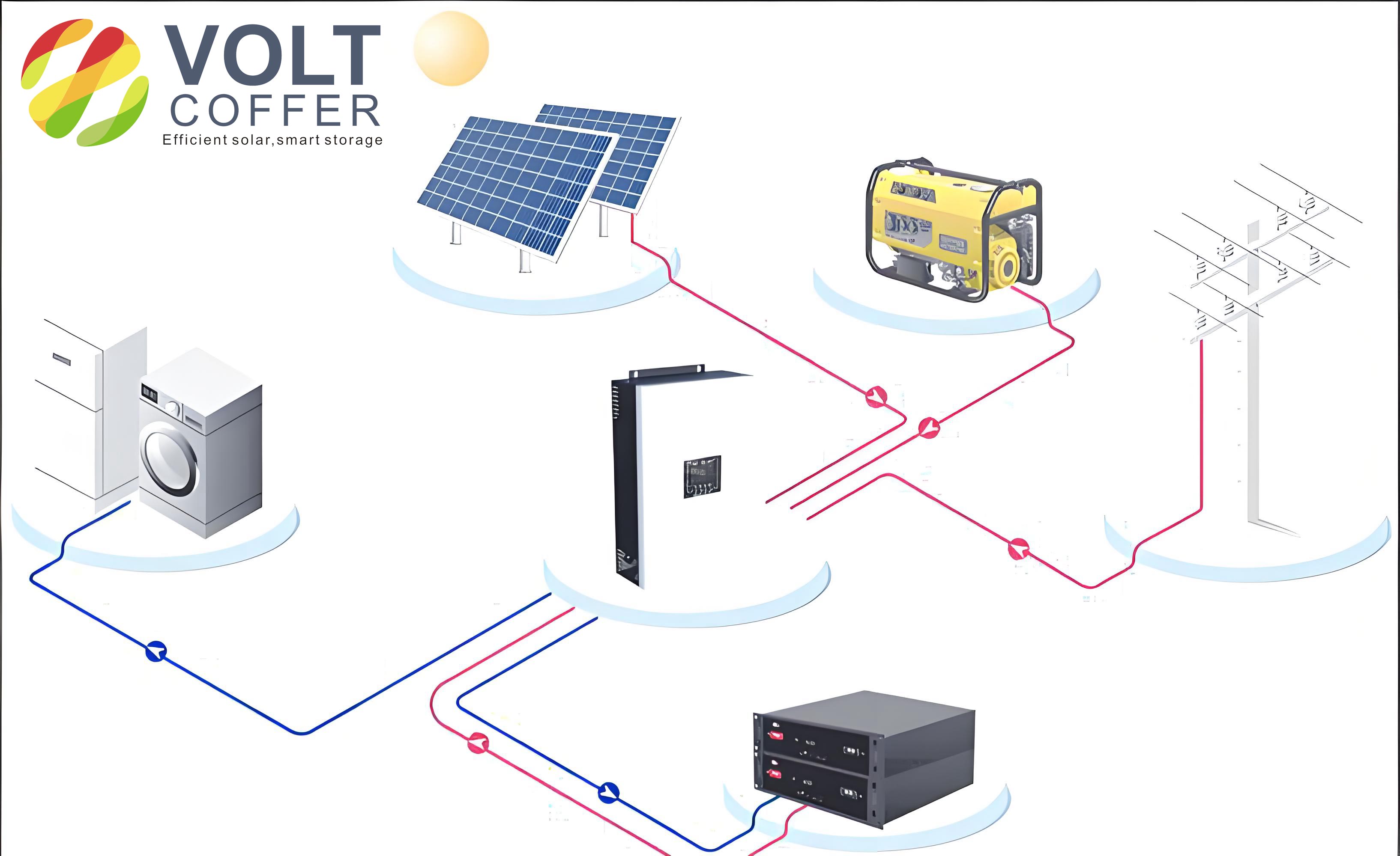
The fundamental structure of an off-grid solar system comprises several key components: photovoltaic (PV) modules, a charge controller, a battery bank, an inverter, and the electrical loads. The PV modules convert solar energy into direct current (DC) electricity. The charge controller regulates the charging and discharging of the battery bank to prevent overcharging or deep discharging, which can degrade battery life. The inverter transforms the DC electricity into alternating current (AC) at 220V, suitable for standard household appliances. The battery bank stores excess energy generated during the day for use during nighttime or periods of low solar irradiance. This configuration ensures a self-sustaining power supply, making it invaluable in areas without grid access. A well-designed off-grid solar system must balance energy generation, storage, and consumption to minimize the risk of power shortages while optimizing cost and longevity.
Designing an off-grid solar system involves a meticulous process that can be executed through manual calculations or specialized software like PVsyst. Manual methods often provide approximate estimates, whereas software tools enable precise optimization by incorporating detailed environmental and load data. The design sequence begins with acquiring local meteorological data, including solar irradiance, temperature, wind speed, atmospheric turbidity, and relative humidity. These parameters are crucial for determining the solar energy potential. The peak sun hours, which represent the equivalent hours of standard irradiance (1 kW/m²), simplify calculations by converting total irradiation into a usable metric. For instance, the daily solar radiation can be expressed in kWh/m², and the peak sun hours (H_{peak}) are derived as:
$$ H_{peak} = \frac{\text{Total Daily Irradiation (kWh/m²)}{1 \text{ kW/m²}} $$
Next, the orientation and tilt angle of the PV modules must be optimized. In the Northern Hemisphere, modules should face south with an azimuth angle of 0°. The tilt angle is typically set to maximize energy capture, often optimized for winter when solar radiation is weakest to avoid power deficits. This is critical for off-grid solar systems, as winter optimization ensures reliability during low-sun periods. The optimal tilt angle (β) can be estimated based on latitude (φ), with adjustments for seasonal variations. For example, a common approximation is β = φ + 15° for winter optimization.
Accurate load profiling is the cornerstone of designing an efficient off-grid solar system. It involves quantifying the energy consumption of all electrical loads over time, considering seasonal and daily variations. Loads should be categorized by power rating, usage duration, and operational periods. For instance, in a forest-based application, loads may include lighting, refrigerators, televisions, washing machines, ventilation fans, and occasional high-power appliances like air conditioners. Table 1 summarizes exemplary seasonal load data for a remote site, illustrating how consumption patterns shift between winter and summer due to factors like daylight hours and cooling needs.
| Load Name | Quantity | Power (W) | Winter Usage (h) | Winter Time Slot | Summer Usage (h) | Summer Time Slot |
|---|---|---|---|---|---|---|
| Lighting | 10 | 10 | 6 | 17:00-23:00 | 4 | 19:00-23:00 |
| Television | 2 | 100 | 6 | 17:00-23:00 | 4 | 19:00-23:00 |
| Refrigerator | 2 | 50 | 24 | All Day | 24 | All Day |
| Washing Machine | 1 | 1000 | 2 | 12:00-14:00 | 2 | 12:00-14:00 |
| Ventilation Fan | 1 | 100 | 24 | All Day | 24 | All Day |
| Small Appliances | 1 | 500 | 6 | 17:00-23:00 | 6 | 17:00-23:00 |
| Standby Devices | 1 | 6 | 24 | All Day | 24 | All Day |
| Air Conditioner | 1 | 1000 | 0 | N/A | 3 | 12:00-15:00 |
Based on the load data, the daily energy consumption (E_{daily}) in watt-hours (Wh) can be calculated as the sum of the products of power and usage time for all loads. For example, in summer, the inclusion of air conditioning significantly increases consumption. The total load energy is given by:
$$ E_{daily} = \sum (P_i \times t_i) $$
where P_i is the power of load i, and t_i is its daily usage time. This value is essential for sizing the PV modules and battery bank. The PV module capacity is determined to meet the daily energy demand, considering losses. The number of parallel strings (N_{parallel}) and the total PV power (P_{total}) are calculated as:
$$ N_{parallel} = \frac{E_{daily}}{E_{gen} \times \eta_{charge} \times \eta_{loss} \times \eta_{inverter}} $$
and
$$ P_{total} = N_{series} \times N_{parallel} \times P_{module} $$
where E_{gen} is the daily energy generation per module, η_{charge} is the charging efficiency (typically 0.9-0.95), η_{loss} accounts for system losses (e.g., soiling, wiring, typically 0.85-0.9), and η_{inverter} is the inverter efficiency (around 0.9-0.95). The daily energy generation per module depends on peak sun hours and module efficiency:
$$ E_{gen} = P_{module} \times H_{peak} \times \eta_{module} $$
For the battery bank, capacity sizing must account for energy storage over consecutive cloudy days and depth of discharge (DOD) to prolong battery life. Lead-acid batteries are commonly used due to their cost-effectiveness, though lithium-ion options offer higher efficiency and longer cycle life. The battery capacity (C) in ampere-hours (Ah) is calculated as:
$$ C = A \times Q_L \times N_L \times T_0 / DOD $$
where A is a safety factor (1.1 to 1.4), Q_L is the daily load in Ah, N_L is the number of autonomous days (e.g., 4 days), T_0 is the temperature correction factor (usually 1 for temperatures above 25°C, but it decreases in colder conditions), and DOD is the maximum allowable discharge depth (typically 0.5 for lead-acid to ensure longevity). The battery voltage (V_{batt}) must match the system voltage, often 48V for larger setups, achieved by series-parallel configurations. The relationship between DOD and cycle life is nonlinear; for instance, lead-acid batteries may endure over 2000 cycles at 40% DOD but only 1000 cycles at 80% DOD.
Controller and inverter selection are based on the system voltage and power ratings. The charge controller must handle the maximum current from the PV array and to the battery, while the inverter’s power rating should exceed the total peak load power. For example, a 48V system requires a 48V controller and inverter. Modern MPPT controllers optimize energy harvest by tracking the maximum power point, improving efficiency compared to PWM types.
To illustrate the design process, I utilized PVsyst software for a case study in a forested region. The site has specific geographical coordinates, and meteorological data was extracted from the Meteonorm database. Table 2 presents the annual meteorological data, which informs the solar resource assessment and system sizing.
| Month | Horizontal Irradiation (kWh/m²) | Horizontal Diffusion (kWh/m²) | Temperature (°C) | Wind Speed (m/s) |
|---|---|---|---|---|
| January | 136.6 | 38.79 | 11.61 | 1.2 |
| February | 136.4 | 45.63 | 14.28 | 1.5 |
| March | 165.2 | 64.17 | 17.41 | 1.6 |
| April | 177.3 | 75.21 | 19.57 | 1.5 |
| May | 179.9 | 71.86 | 21.48 | 1.3 |
| June | 124.4 | 79.81 | 22.21 | 1.3 |
| July | 130.5 | 73.04 | 22.26 | 1.1 |
| August | 141.1 | 77.13 | 22.44 | 1.2 |
| September | 124.7 | 74.78 | 21.24 | 1.2 |
| October | 123.8 | 60.73 | 19.32 | 1.1 |
| November | 131.2 | 44.92 | 15.19 | 1.1 |
| December | 128.7 | 30.94 | 12.25 | 1.1 |
The optimal tilt angle was set to 44° for winter optimization, maximizing energy capture during the low-sun season. Load data analysis revealed an average daily energy consumption of 11 kWh, with higher usage in summer due to air conditioning. The off-grid solar system was designed with a target loss of load probability (LOLP) of 5%, meaning the system should meet load demands 95% of the time. Using PVsyst, the simulation recommended a PV array capacity of 4469 Wp and a battery capacity of 1239 Ah at 48V.
For component selection, I chose monocrystalline silicon PV modules with a peak power of 230 W each. The array configuration involved 4 series strings and 4 parallel strings, totaling 16 modules and 4600 Wp. The battery bank comprised lead-acid batteries, each 12V and 239 Ah, arranged in 4 series and 5 parallel strings to achieve 48V and 1195 Ah. A single MPPT charge controller with a 65A charging current and a 48V inverter were selected to match the system specifications.
Simulation results from PVsyst provided insights into system performance. The normalized energy production and loss diagram indicated that PV array losses accounted for 17.9%, system and battery losses were 5.3%, and 29.4% of the generated energy was unused surplus, primarily in spring, autumn, and winter. However, in summer, particularly July, the surplus diminished, and a power deficit occurred due to air conditioner usage. The system efficiency and solar fraction analysis showed that the off-grid solar system could supply 100% of the load in spring, autumn, and winter, but only 90% in summer, corresponding to a 10% loss of load probability. This underscores the impact of seasonal load variations on the reliability of off-grid solar systems.
The battery state of charge (SOC) profile further highlighted system behavior. In non-summer months, the SOC remained around 85%, with a daily discharge depth of 15%, which is ideal for battery longevity. In contrast, from June to September, the SOC dropped to approximately 40%, necessitating deeper discharges that could reduce battery cycle life. Nevertheless, the overall annual performance suggests that such deep discharges are infrequent, minimizing long-term degradation. This analysis demonstrates the importance of sizing the off-grid solar system to handle peak demands while maintaining battery health.
In conclusion, the optimization of an off-grid solar system relies heavily on detailed load data and meteorological analysis. This paper has outlined a comprehensive design approach, incorporating software tools like PVsyst for precision. The case study illustrates that while the system generally meets user needs, seasonal fluctuations—especially summer cooling demands—can lead to temporary power shortages. Future optimizations could involve adjusting the tilt angle for summer efficiency or increasing battery capacity to enhance reliability. Ultimately, a well-designed off-grid solar system offers a sustainable energy solution for remote applications, contributing to carbon reduction goals. Continued advancements in PV technology and energy storage will further improve the viability of such systems, making them indispensable in the global energy landscape.