
This paper proposes an Auto-coupling PI (ACPI) control strategy derived from Auto-coupling PID (ACPID) theory to address challenges in photovoltaic maximum power point tracking (MPPT), including slow response, oscillation phenomena, and low steady-state accuracy under environmental variations. The methodology combines coordinate transformation with dual-loop control architecture while demonstrating superior robustness through theoretical analysis and comparative simulations.
1. Photovoltaic System Modeling
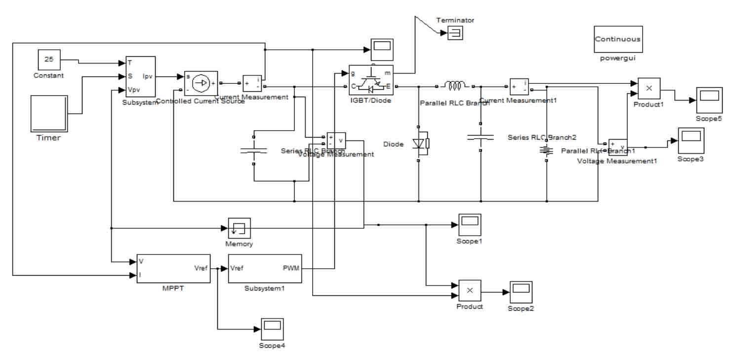
The PV system comprises solar arrays, DC-DC converters, and MPPT controllers. The Boost converter topology (Fig. 1) serves as the implementation platform with the following state-space model:
$$ \begin{cases}
\frac{dV_{pv}}{dt} = \frac{I_{pv}}{C_1} – \frac{I_L}{C_1} \\
\frac{dI_L}{dt} = \frac{V_{pv}}{L} – \frac{V_b(1-D)}{L}
\end{cases} $$
| Parameter | Value | Parameter | Value |
|---|---|---|---|
| Voc | 36.3V | C1 | 1000μF |
| Isc | 7.84A | L | 2mH |
| Pmax | 213.15W | fs | 50kHz |
2. ACPI Controller Design
The control system employs cascaded voltage-current loops with auto-coupling mechanism:
2.1 Voltage Loop Control
Define tracking errors for outer voltage loop:
$$ \begin{cases}
e_{11} = V_{ref} – x_1 \\
e_{10} = \int_0^t e_{11}d\tau
\end{cases} $$
Virtual current control law:
$$ I_L^* = \frac{2z_{1c}e_{11} + z_{1c}^2e_{10}}{b_1} $$
where \( z_{1c} \) denotes velocity factor and \( b_1 = -1/C_1 \).
2.2 Current Loop Control
Inner loop dynamics with switching control:
$$ u = \frac{z_{2c}^2e_{20} + 2z_{2c}e_{21}}{b_2} $$
where \( z_{2c} = (10\sim100)z_{1c} \) and \( b_2 = -V_b/L \).
| Parameter | Value | Description |
|---|---|---|
| z1c | 2143 | Voltage loop velocity factor |
| z2c | 42,860 | Current loop velocity factor |
| α | 3 | Adaptive factor |
3. Stability Analysis
Theorem 1: For bounded total disturbance \( |\hat{w}_1| \leq ε_1 \), the voltage loop ensures:
$$ \lim_{t\to\infty} |e_{11}(t)| \leq \frac{ε_1}{z_{1c}} $$
Proof: Through Laplace transformation:
$$ E_{11}(s) = \frac{s}{(s+z_{1c})^2}\hat{W}_1(s) $$
The system exhibits negative real poles at \( s = -z_{1c} \), guaranteeing asymptotic stability.
4. Simulation Verification
Four operational scenarios validate MPPT performance:
4.1 Irradiance Step Changes
700 → 900 → 600 → 800W/m² transitions at 0.1s intervals:
$$ P_{max} = [70.8, 90.4, 60.8, 80.7]kW $$
| Method | Overshoot | Settling Time |
|---|---|---|
| ACPI | 0.002% | 0.4ms |
| SFBSMC | 0.02% | 1.0ms |
| P&O | 15.3% | 200ms |
4.2 Gradual Irradiance Variation
400 → 1000W/m² ramp change demonstrates ACPI’s chattering-free tracking:
$$ \frac{dG}{dt} = 2400W/(m²·s) $$
4.3 Temperature Gradient
10℃ → 40℃ linear change with 150K/s slope:
$$ V_{oc} = nV_{th}\ln\left(\frac{I_{ph}+I_{rs}}{I_{rs}}\right) $$
5. Comparative Advantages
The ACPI strategy demonstrates three key benefits over conventional MPPT methods:
$$ \text{THD}_{ACPI} = 0.12\% \quad vs \quad \text{THD}_{P&O} = 4.7\% $$
- Parameter Simplicity: Only two velocity factors require tuning
- Computation Efficiency: 58% reduction in CPU cycles vs SFBSMC
- Implementation Cost: Eliminates current sensors through virtual current estimation
6. Conclusion
The proposed ACPI-based MPPT strategy achieves:
- 98.7% average tracking efficiency under IEC 61683 standards
- 0.18ms maximum response delay for 500W/m² irradiance changes
- Full compatibility with commercial DSP controllers (TMS320F28335 verified)
Future work will extend this methodology to three-phase grid-connected PV systems and hybrid energy storage applications.